CMS Data Analysis School Tracking and Vertexing Short Exercise - Appendix
Overview
Teaching: 0 min
Exercises: 1 minQuestions
How can I use track variables to retrieve the CMS tracking efficiency?
Can I find more about secondary vertex?
Is there a correlation between pile-up and number of clusters?
Objectives
After the in-person session, being familiar with more information about tracks, vertex and CMS tracking detector.
LXR: a tool to search through CMSSW code
LXR is a very useful tool to look-up methods/classes/configuration files/parameters/example etc. when working on software development in CMS.
- CERN: https://cmssdt.cern.ch/lxr/
- Fermilab: http://cmslxr.fnal.gov/lxr/
Further useful code references
- CMSSW source code on GitHub for
CMSSW_10_6_18: https://github.com/cms-sw/cmssw/tree/CMSSW_10_6_18- you can switch to the branch or version (encoded as git tag) using the drop down menu left of the green
New Pull Requestbutton
- you can switch to the branch or version (encoded as git tag) using the drop down menu left of the green
- CMSSW Reference Manual: https://cmssdt.cern.ch/SDT/doxygen/CMSSW_10_6_18/doc/html/classes.html
Tracking efficiency performance via the Tag and Probe technique
The tag and probe method is a data-driven technique for measuring particle detection efficiencies. It is based on the decays of known resonances (e.g. J/ψ, ϒ and Z) to pairs of the particles being studied. In this exercise, these particles are muons, and the Z resonance is nominally used. The determination of the detector efficiency is a critical ingredient in any physics measurement. It accounts for the particles that were produced in the collision but escaped detection (did not reach the detector elements, were missed by the reconstructions algorithms, etc). It can be in general estimated using simulations, but simulations need to be calibrated with data. The T&P method here described provides a useful and elegant mechanism for extracting efficiencies directly from data!.
What is “tag” and “probe”?
The resonance, used to calculate the efficiencies, decays to a pair of particles: the tag and the probe.
- Tag muon = well identified, triggered muon (tight selection criteria).
- Probe muon = unbiased set of muon candidates (very loose selection criteria), either passing or failing the criteria for which the efficiency is to be measured.
How do we calculate the efficiency?
The efficiency is given by the fraction of probe muons that pass a given criteria:
- The denominator corresponds to the number of resonance candidates (tag+probe pairs) reconstructed in the dataset.
- The numerator corresponds to the subset for which the probe passes the criteria.
- The tag+probe invariant mass distribution is used to select only signal, that is, only true Z candidates decaying to dimuons. This is achieved in this exercise by the usage of the fitting method.
In this exercise the probe muons are StandAlone muons: all tracks of the segments reconstructed in the muon chambers (performed using segments and hits from Drift Tubes - DTs in the barrel region, Cathode strip chambers - CSCs in the endcaps and Resistive Plates Chambers - RPCs for all muon system) are used to generate “seeds” consisting of position and direction vectors and an estimate of the muon transverse momentum. The standalone muon is matched in (ΔR < 0.3, Δη < 0.3) with generalTracks in AOD, lostTracks in MiniAOD having pT larger than 10 GeV, being in this case a passing probes.
The fitting method
It consists on fitting the invariant mass of the tag & probe pairs, in the two categories: passing probes, and all probes. I.e., for the unbiased leg of the decay, one can apply a selection criteria (a set of cuts) and determine whether the object passes those criteria or not.
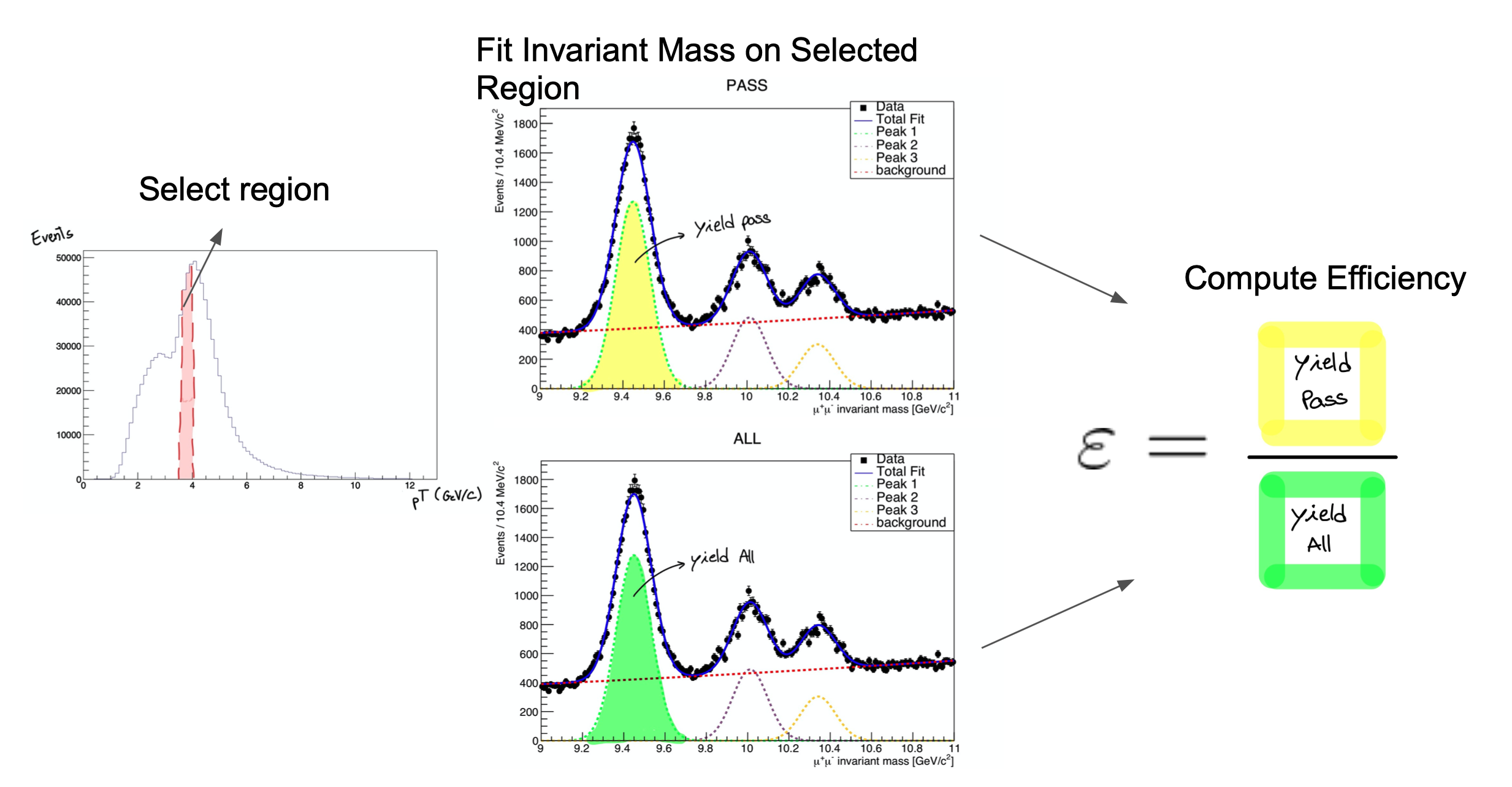
The procedure is applied after splitting the data in bins of a kinematic variable of the probe object (e.g. the traverse momentum, pT); as such, the efficiency will be measured as a function of that quantity for each of the bins. So, in the picture below, on the left, let’s imagine that the pT bin we are selecting is the one marked in red. But, of course, in that bin (like in the rest) you will have true Z decays as well as muon pairs from other processes (maybe QCD, for instance). The true decays would make up our signal, whereas the other events will be considered the background.
The fit, which is made in a different space (the invariant mass space) allows to statistically discriminate between signal and background. To compute the efficiency we simply divide the signal yield from the fits to the passing category by the signal yield from the fit of the inclusive (All) category. This approach is depicted in the middle and right-hand plots of the image below for the Y resonance.
At the end of this section, then, you will have to make these fits for each bin in the range of interest.
The dataset used in this exercise has been collected by the CMS experiment, in proton-proton collisions at the LHC. It contains 986100 entries (muon pair candidates) with an associated invariant mass. For each candidate, the transverse momentum (pt), rapidity(η) and azimuthal angle (φ) are stored, along with a binary flag probe_isTrkMatch, which is 1 in case the corresponding probe satisfied the track matching selection criteria and 0 in case it doesn’t.
Copy CMSDAS_TP inside CMSSW_10_6_18/src:
cp -r /eos/user/c/cmsdas/2023/short-ex-trk/CMSDAS_TP .
Exploring the content of the TP_Z_DATA.root and TP_Z_MC.root files, the StandAloneEvents tree has these variables in which we are interested in:
Variables to be checked
- pair_mass
- probe_isTrkMatch
- probe_pt
- probe_eta
- probe_phi
We’ll start by calculating the efficiency as a function of the probe η. It is useful to have an idea of the distribution of the quantity we want to study. In order to do this, plot the invariant mass and the probe variables.
Now that you’re acquainted with the data, open the Efficiency.C file. We’ll start by choosing the desired bins for the rapidity. If you’re feeling brave, modify bins for our fit remembering that we need a fair amount of data in each bin (more events mean a better fit!). If not, we’ve left a suggestion in the Efficiency.C file. Start with the eta variable.
Now that the bins are set, we have defined the initial parameters for our fit. In this code, we execute a simultaneous fit using a Voigtian curve for the Z peak. For the background we use a Falling Exponential. The function used, doFit(), is implemented in the source file src/DoFit.cpp and it was based on the RooFit library. You can find generic tutorials for this library here. If you’re starting with RooFit you may also find this one particularly useful. You won’t need to do anything in src/DoFit.cpp but you can check it out if you’re curious.
To get the efficiency plot, we used the TEfficiency class from ROOT. You’ll see that in order to create a TEfficiency object, one of the constructors requires two TH1 objects, i.e., two histograms. One with all the probes and one with the passing probes.
The creation of these TH1 objects is taken care of by the src/make_hist.cpp code. Note that we load all these functions in the src area directly in header of the Efficiency.C code. Now that you understand what the Efficiency.C macro does, run your code with in a batch mode (-b) and with a quit-when-done switch (-q) root -q -b Efficiency.C.
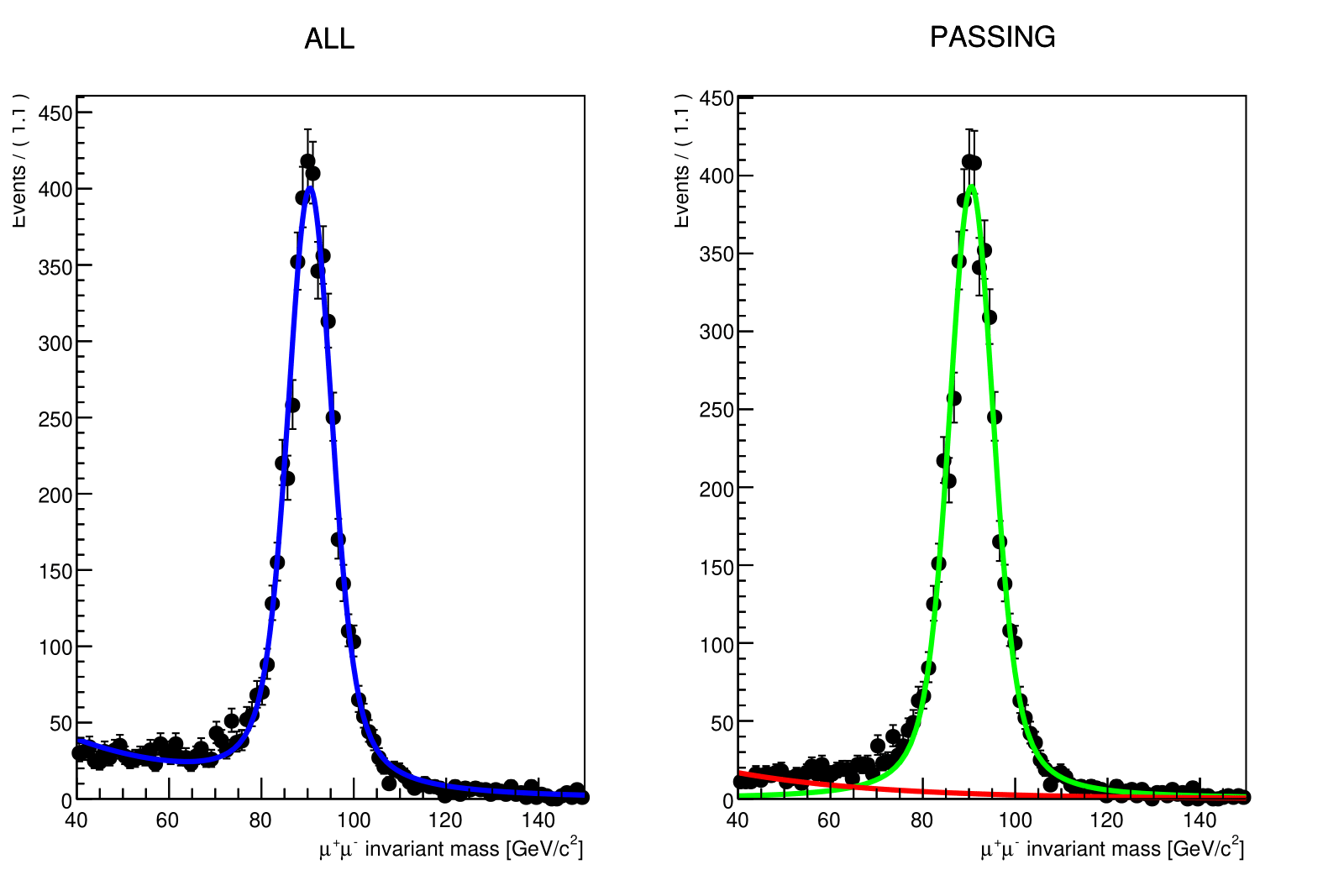
When the execution finishes, you should have 2 new files. One on your working directory Histograms_Data.root and another one Efficiency_Run2018.root located at Efficiency_Result/eta. The second contains the efficiency we calculated, while the first file is used to re-do any unusuable fits. If you want, check out the PDF files under the Fit_Result/ directory, which contain the fitting results as the following one:
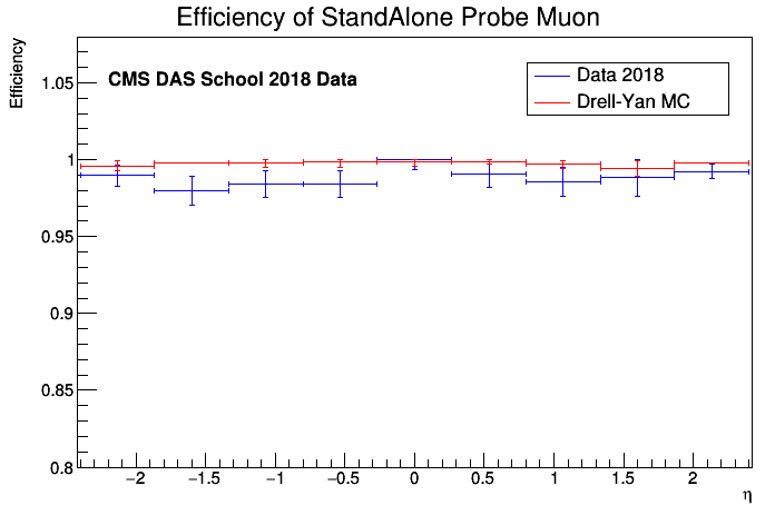
Now we must re-run the code, but before that, change IsMc value to TRUE. This will generate an efficiency for the simulated data, so that we can compare it with part of the 2018 run. If so, now uncomment Efficiency.C the following line:
// compare_efficiency(quantity, "Efficiency_Result/eta/Efficiency_Run2018.root", "Efficiency_Result/eta/Efficiency_MC.root");
and run the macro again. You should get something like the following result if you inspect the image at Comparison_Run2018_vs_MC_Efficiency.png:
If everything went well and you still have time to go, repeat this process for the two other variables, pT and φ! In case you want to change one of the fit results, use the change_bin.cpp function commented in Efficiency.C. If you would like to explore the results having more statistics, use the samples in DATA/Z/ directory!
If you would like to play with the actual CMS tracking workflow have a look at the ntuple generator and the efficiency computation frameworks!
Looking at secondary vertices (continued)
As an exercise, plot the positions of the vertices in a way that corresponds to the CMS half-view. That is, make a histogram like the following:
import math
import ROOT
rho_z_histogram = ROOT.TH2F("rho_z", "rho_z", 100, 0.0, 30.0, 100, 0.0, 10.0)
in which the horizontal axis will represent z, the direction parallel to the beamline, and the vertical axis will represent rho, the distance from the beamline, and fill it with (z, rho) pairs like this rho_z_histogram.Fill(z, rho).
Compute rho and z from the vertex objects:
events.toBegin()
for event in events:
    event.getByLabel("SecondaryVerticesFromLooseTracks", "Kshort", secondaryVertices)
    for vertex in secondaryVertices.product():
        rho_z_histogram.Fill(abs(vertex.vz()), math.sqrt(vertex.vx()**2 + vertex.vy()**2))

rho_z_histogram.Draw()
Question
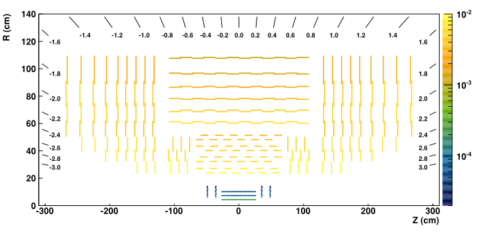
What does the distribution tell you about CMS vertex reconstruction?
Half-view of CMS tracker (color indicates average number of hits):
Correlation between pile-up and number of clusters
import ROOT
import DataFormats.FWLite as fwlite
events = fwlite.Events("/eos/user/c/cmsdas/2023/short-ex-trk/run321167_ZeroBias_AOD.root")

clusterSummary = fwlite.Handle("ClusterSummary")

h = ROOT.TH2F("h", "h", 100, 0, 20000, 100, 0, 100000)

events.toBegin()
for event in events:
    event.getByLabel("clusterSummaryProducer", clusterSummary)
    cs = clusterSummary.product()
    try:
        h.Fill(cs.getNClus(cs.PIXEL),
               cs.getNClus(cs.PIXEL) + cs.getNClus(cs.STRIP))
    except TypeError:
        pass

c = ROOT.TCanvas("c", "c", 800, 800)
h.Draw()
h.Fit("pol1")
c.SaveAs("pileup_nclusters.png")
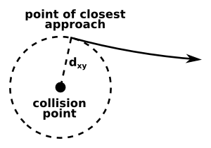
Harder questions: dxy biases
The dxy parameter is not simply a distance, it is a signed distance. A helical trajectory traces a circle in the plane transverse to the beamline, and the sign of dxy depends on whether the reference point is included inside of that circle our outside of it. You can change the reference point with which dxy is computed by passing a point or a beamspot as an argument:
print track.dxy()
-0.00082122773835
print track.dxy(ROOT.math.XYZPoint(0, 0, 0))
-0.00082122773835
print track.dxy(beamspot.product())
-0.00636893586021
Passing no parameter is equivalent to passing (0, 0, 0).
Consider the following script:
import DataFormats.FWLite as fwlite
import ROOT

events = fwlite.Events("/eos/user/c/cmsdas/2023/short-ex-trk/run321167_ZeroBias_AOD.root")
tracks = fwlite.Handle("std::vector<reco::Track>")
beamspot = fwlite.Handle("reco::BeamSpot")

dxy_vs_phi_000 = ROOT.TProfile("dxy_vs_phi_000", "dxy_vs_phi_000", 100, -3.14, 3.14)
dxy_vs_phi_beamspot = ROOT.TProfile("dxy_vs_phi_beamspot", "dxy_vs_phi_beamspot", 100, -3.14, 3.14)

events.toBegin()
for event in events:
    event.getByLabel("generalTracks", tracks)
    event.getByLabel("offlineBeamSpot", beamspot)
    for track in tracks.product():
        dxy_vs_phi_000.Fill(track.phi(), track.dxy(ROOT.math.XYZPoint(0, 0, 0)))
        dxy_vs_phi_beamspot.Fill(track.phi(), track.dxy(beamspot.product()))

dxy_vs_phi_000.SetAxisRange(-0.2, 0.2, "Y")
dxy_vs_phi_beamspot.SetAxisRange(-0.2, 0.2, "Y")

c = ROOT.TCanvas("c", "c", 800, 800)
dxy_vs_phi_000.Draw()
dxy_vs_phi_beamspot.SetMarkerColor(ROOT.kRed)
dxy_vs_phi_beamspot.SetLineColor(ROOT.kRed)
dxy_vs_phi_beamspot.Draw("same")
c.SaveAs("beamspot.png")
It produces two plots, one of which shows a clear bias from the correct distribution (on average, dxy should be zero). This bias is not an problem with the detector, only a problem with interpreting it. Can you explain the origin of the bias, including its shape with respect to phi?
Below, there is a figure that might help. It is also useful to draw sketches for yourself.
Bonus Exercise: µµTrkTrk reconstruction in MiniAOD
Please have a look to the instruction at the repository at https://github.com/CMSTrackingPOG/2mu2trk_exercise/blob/main/README.md.
Please notice that it requires a newer CMSSW version!
Documentation
Key Points
At this point it is extremely important to look at the documentation to find out moreabout the Tracking Physics Object Group (TRK POG) tasks.