CMS Data Analysis School Tracking and Vertexing Short Exercise - The five basic track variables

Overview

Teaching: 15 min
Exercises: 15 min

Questions

What are the main track variables used in CMS collaboration in different data formats?

How can we access them?

Which are the track quality variables?

How do the distributions of track variables before and after high purity track selection change?

Objectives

Being familiar with tracks collections and their variables.

Being aware of track information stored in different data format.

Accessing information and plot basic variables using ROOT.

One of the oldest tricks in particle physics is to put a track-measuring device in a strong, roughly uniform magnetic field so that the tracks curve with a radius proportional to their momenta (see derivation). Apart from energy loss and magnetic field inhomogeneities, the particles’ trajectories are helices. This allows us to measure a dynamic property (momentum) from a geometric property (radius of curvature).

A helical trajectory can be expressed by five parameters, but the parameterization is not unique. Given one parameterization, we can always re-express the same trajectory in another parameterization. Many of the data fields in a CMSSW reco::Track are alternate ways of expressing the same thing, and there are functions for changing the reference point from which the parameters are expressed. (For a much more detailed description, see this page.)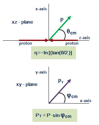

The five basic track parameters

signed radius of curvature (units of cm), which is proportional to particle charge divided by the transverse momentum, p_T (units of GeV);

angle of the trajectory at a given point on the helix, in the plane transverse to the beamline (usually called φ);

angle of the trajectory at a given point on the helix with respect to the beamline (θ, or equivalently λ = π/2 - θ), which is usually expressed in terms of pseudorapidity (η = −ln(tan(θ/2)));

offset or impact parameter relative to some reference point (usually the beamspot or a selected primary vertex), in the plane transverse to the beamline (usually called dxy);

impact parameter relative to a reference point (beamspot or a selected primary vertex), along the beamline (usually called dz).

The exact definitions are given in the reco::TrackBase header file. This is also where most tracking variables and functions are defined. The rest are in the reco::Track header file, but most data fields in the latter are accessible only in RECO (full data record), not AOD/MiniAOD/NanoAOD (the subsets that are available to physics analyses).

Accessing track variables

Create print.py (for example emacs -nw print.py, or use your favorite text editor) in TrackingShortExercize/, then copy-paste the following code and run it (python print.py). Please note, if your run321457_ZeroBias_AOD.root is not in the directory you’re working from, be sure to use the appropriate path in line 2.

import DataFormats.FWLite as fwlite
events = fwlite.Events("/eos/user/c/cmsdas/2023/short-ex-trk/run321167_ZeroBias_AOD.root")
tracks = fwlite.Handle("std::vector<reco::Track>")

for i, event in enumerate(events):
    if i >= 5: break # print info only about the first 5 events
    print "Event", i
    event.getByLabel("generalTracks", tracks)
    for j, track in enumerate(tracks.product()):
        print "    Track", j,
        print "\t charge/pT: %.3f" %(track.charge()/track.pt()),
        print "\t phi: %.3f" %track.phi(),
        print "\t eta: %.3f" %track.eta(),
        print "\t dxy: %.4f" %track.dxy(),
        print "\t dz: %.4f"  %track.dz()

The first three lines load the FWLite framework, the .root data file, and prepare a Handle for the track collection using its full C++ name (std::vector). In each event, we load the tracks labeled generalTracks and loop over them, printing out the five basic track variables for each. The C++ equivalent of this is hidden below (longer and more difficult to write and compile, but faster to execute on large datasets) and is optional for this entire short exercise.

C++ version
cd ${CMSSW_BASE}/src
mkdir MyDirectory
cd MyDirectory
mkedanlzr PrintOutTracks
cd ..
Use your favorite editor to add (if missing) the following line at the top of MyDirectory/PrintOutTracks/plugins/BuildFile.xml (e.g. emacs -nw MyDirectory/PrintOutTracks/plugins/BuildFile.xml):
<use name="DataFormats/TrackReco"/>
Now edit MyDirectory/PrintOutTracks/plugins/PrintOutTracks.cc and put (if missing) the following in the #include section:
#include <iostream>
#include "DataFormats/TrackReco/interface/Track.h"
#include "DataFormats/TrackReco/interface/TrackFwd.h"
#include "FWCore/Utilities/interface/InputTag.h"
Inside the PrintOutTracks class definition (one line below the member data comment, before the };), replace edm::EDGetTokenT<TrackCollection> tracksToken_; with:
edm::EDGetTokenT<edm::View<reco::Track> > tracksToken_;  //used to select which tracks to read from configuration file
int indexEvent_;
Inside the PrintOutTracks::PrintOutTracks(const edm::ParameterSet& iConfig) constructor before the {, modify the consumes statement to read:
: 
tracksToken_(consumes<edm::View<reco::Track> >(iConfig.getUntrackedParameter<edm::InputTag>("tracks", edm::InputTag("generalTracks")) ))
after the //now do what ever initialization is needed comment:
indexEvent_ = 0;
Put the following inside the PrintOutTracks::analyze method:
  std::cout << "Event " << indexEvent_ << std::endl;

  edm::Handle<edm::View<reco::Track> > trackHandle;
  iEvent.getByToken(tracksToken_, trackHandle);
  if ( !trackHandle.isValid() ) return;
  const edm::View<reco::Track>& tracks = *trackHandle;
  size_t iTrack = 0;
  for ( auto track : tracks ) {
    std::cout << "    Track " << iTrack << " "
       << track.charge()/track.pt() << " "
              << track.phi() << " "
              << track.eta() << " "
              << track.dxy() << " "
              << track.dz()
       << std::endl;
    iTrack++;
  }
  ++indexEvent_;
Now compile it by running:
scram build -j 4
Go back to TrackingShortExercize/ and create a CMSSW configuration file named run_cfg.py (emacs -nw run_cfg.py):
import FWCore.ParameterSet.Config as cms

process = cms.Process("RUN")

process.source = cms.Source("PoolSource",
    fileNames = cms.untracked.vstring("file:/eos/user/c/cmsdas/2023/short-ex-trk/run321167_ZeroBias_AOD.root"))
process.maxEvents = cms.untracked.PSet(input = cms.untracked.int32(5))

process.MessageLogger = cms.Service("MessageLogger",
    destinations = cms.untracked.vstring("cout"),
    cout = cms.untracked.PSet(threshold = cms.untracked.string("ERROR")))

process.PrintOutTracks = cms.EDAnalyzer("PrintOutTracks")
process.PrintOutTracks.tracks = cms.untracked.InputTag("generalTracks")

process.path = cms.Path(process.PrintOutTracks)
And, finally, run it with:
cmsRun run_cfg.py
This will produce the same output as the Python script, but it can be used on huge datasets. Though the language is different, notice that C++ and FWLite use the same names for member functions: charge(), pt(), phi(), eta(), dxy(), and dz(). That is intentional: you can learn what kinds of data are available with interactive FWLite and then use the same access methods when writing GRID jobs. There is another way to access FWLite with ROOT’s C++-like syntax.

The plugin is here: /eos/user/c/cmsdas/2023/short-ex-trk/MyDirectory/PrintOutTracks/plugins/PrintOutTracks.cc The run_cfg.py is here: /eos/user/c/cmsdas/2023/short-ex-trk/MyDirectory/PrintOutTracks/test/run_cfg.py

Track quality variables

The first thing you should notice is that each event has hundreds of tracks. That is because hadronic collisions produce large numbers of particles and generalTracks is the broadest collection of tracks identified by CMSSW reconstruction. Some of these tracks are not real (ghosts, duplicates, noise…) and a good analysis should define quality cuts to select tracks requiring a certain quality. Some analyses remove spurious tracks by requiring them to come from the beamspot (small dxy, dz). Some require high-momentum (usually high transverse momentum, p_T), but that would be a bad idea in a search for decays with a small mass difference such as ψ’ → J/ψ π⁺π^-. In general, each analysis group should review their own needs and ask the Tracking POG about standard selections. 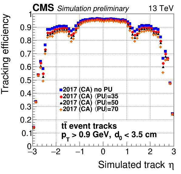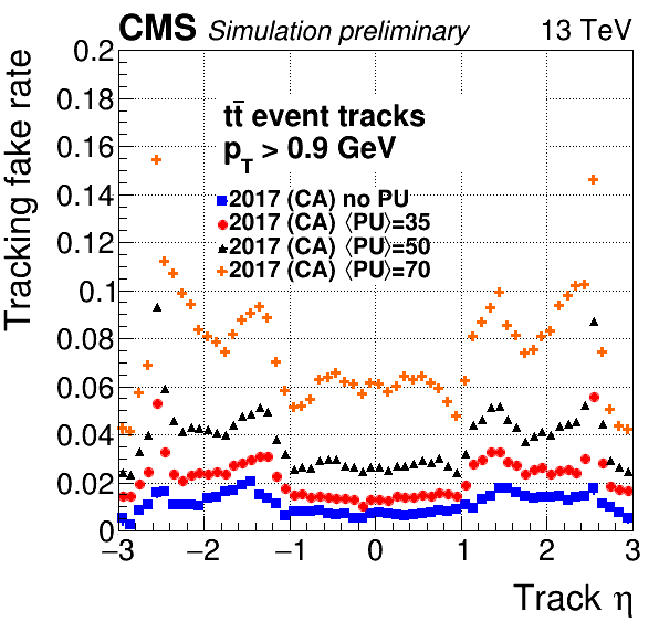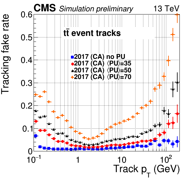Some of these standard selections have been encoded into a quality flag with three categories: loose, tight, and highPurity. All tracks delivered to the analyzers are at least loose, tight is a subset of these that are more likely to be real, and highPurity is a subset of tight with even stricter requirements. There is a trade-off: loose tracks have high efficiency but also high backgrounds, highPurity has slightly lower efficiency but much lower backgrounds, and tight is in between (see also the plots below). As of CMSSW 7.4, these are all calculated using MVAs (MultiVariate Analysis techniques) for the various iterations. In addition to the status bits, it’s also possible to access the MVA values directly.

Plot of Efficiency vs Eta:

Plot of Efficiency vs p_T:

Plot of Backgrounds vs Eta:

Plot of Backgrounds vs p_T:

Update the (create a new) print.py file with the following lines: Add a Handle to the MVA values:

import DataFormats.FWLite as fwlite
events = fwlite.Events("/eos/user/c/cmsdas/2023/short-ex-trk/run321167_ZeroBias_AOD.root")
tracks = fwlite.Handle("std::vector<reco::Track>")
MVAs = fwlite.Handle("std::vector<float>")

The event loop should be updated to this:

for i, event in enumerate(events):
    if i >= 5: break            # only the first 5 events
    print "Event", i
    event.getByLabel("generalTracks", tracks)
    event.getByLabel("generalTracks", "MVAValues", MVAs)

    numTotal = tracks.product().size()
    if numTotal == 0: continue
    numLoose = 0
    numTight = 0
    numHighPurity = 0

    for j, (track, mva) in enumerate(zip(tracks.product(), MVAs.product())):
        if track.quality(track.qualityByName("loose")):      numLoose      += 1
        if track.quality(track.qualityByName("tight")):      numTight      += 1
        if track.quality(track.qualityByName("highPurity")): numHighPurity += 1

        print "    Track", j,
        print "\t charge/pT: %.3f" %(track.charge()/track.pt()),
        print "\t phi: %.3f" %track.phi(),
        print "\t eta: %.3f" %track.eta(),
        print "\t dxy: %.4f" %track.dxy(),
        print "\t dz: %.4f"  %track.dz(),
        print "\t nHits: %s" %track.numberOfValidHits(), "(%s P+ %s S)"%(track.hitPattern().numberOfValidPixelHits(),track.hitPattern().numberOfValidStripHits()),
        print "\t algo: %s"  %track.algoName(),
        print "\t mva: %.3f" %mva

    print "Event", i,   
    print "numTotal:", numTotal,
    print "numLoose:", numLoose, "(%.1f %%)"%(float(numLoose)/numTotal*100),
    print "numTight:", numTight, "(%.1f %%)"%(float(numTight)/numTotal*100),  
    print "numHighPurity:", numHighPurity, "(%.1f %%)"%(float(numHighPurity)/numTotal*100)

The C++-equivalent is hidden below.

C++ version

Update your EDAnalyzer adding the following lines:

To class declaration:

edm::EDGetTokenT<edm::View<float> > mvaValsToken_;

To constructor:

, mvaValsToken_( consumes<edm::View<float> >(iConfig.getUntrackedParameter<edm::InputTag>("mvaValues", edm::InputTag("generalTracks", "MVAValues")) ) )

Change your analyze method to:

  std::cout << "Event " << indexEvent_ << std::endl;

  edm::Handle<edm::View<reco::Track> > trackHandle;
  iEvent.getByToken(tracksToken_, trackHandle);
  if ( !trackHandle.isValid() ) return;
  const auto numTotal = trackHandle->size();

  edm::Handle<edm::View<float> > trackMVAstoreHandle;
  iEvent.getByToken(mvaValsToken_,trackMVAstoreHandle);
  if ( !trackMVAstoreHandle.isValid() ) return;

  auto numLoose = 0;
  auto numTight = 0;
  auto numHighPurity = 0;

  const edm::View<reco::Track>& tracks = *trackHandle;
  size_t iTrack = 0;
  for ( auto track : tracks ) {
    if (track.quality(track.qualityByName("loose"))     ) ++numLoose;
    if (track.quality(track.qualityByName("tight"))     ) ++numTight;
    if (track.quality(track.qualityByName("highPurity"))) ++numHighPurity;

    std::cout << "    Track " << iTrack << " "
       << track.charge()/track.pt() << " "
              << track.phi() << " "
              << track.eta() << " "
              << track.dxy() << " "
              << track.dz()
              << track.chi2() << " "
       << track.ndof() << " "
              << track.numberOfValidHits() << " "
              << track.algoName() << " "
              << trackMVAstoreHandle->at(iTrack)
              << std::endl;
    iTrack++;
  }
  ++indexEvent_;

  std::cout << "Event " << indexEvent_
            << " numTotal: " << numTotal
            << " numLoose: " << numLoose
            << " numTight: " << numTight
            << " numHighPurity: " << numHighPurity
            << std::endl;

Go back to TrackingShortExercize/ and edit the CMSSW configuration file named run_cfg.py (emacs -nw run_cfg.py), adding the following line:

process.PrintOutTracks.mvaValues = cms.untracked.InputTag("generalTracks","MVAValues")

Now run the analyzer:

cmsRun run_cfg.py

The plugin can be found in /eos/user/c/cmsdas/2023/short-ex-trk/PrintOutTracks_MVA.cc The CMSSW config file can be found in /eos/user/c/cmsdas/2023/short-ex-trk/run_cfg_MVA.py

Question 1

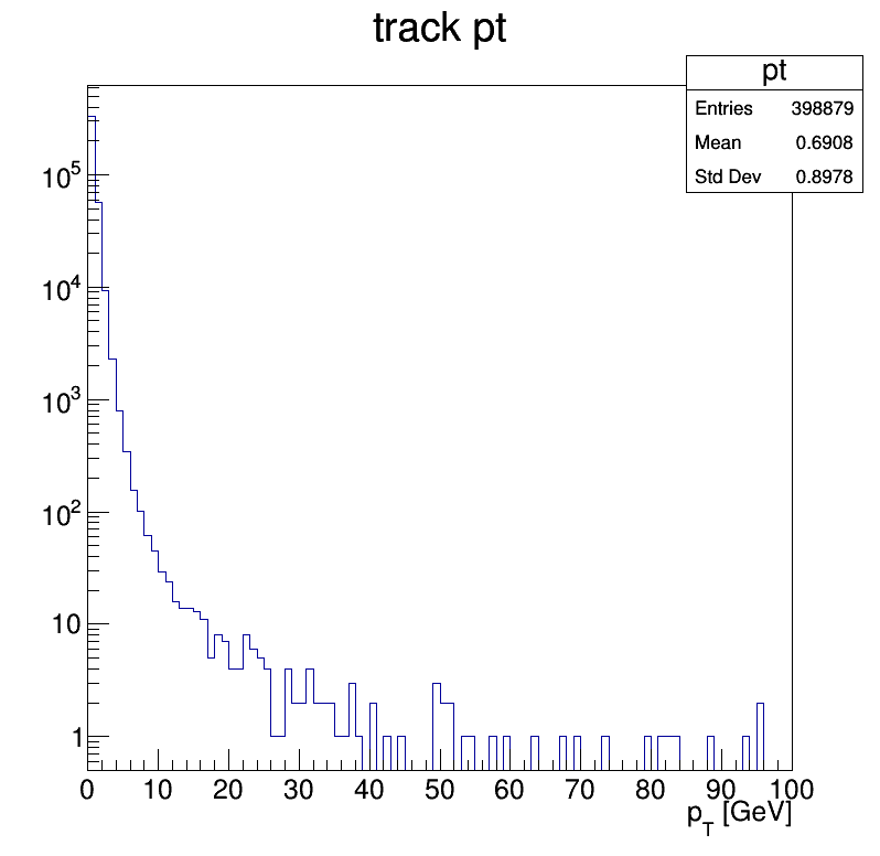
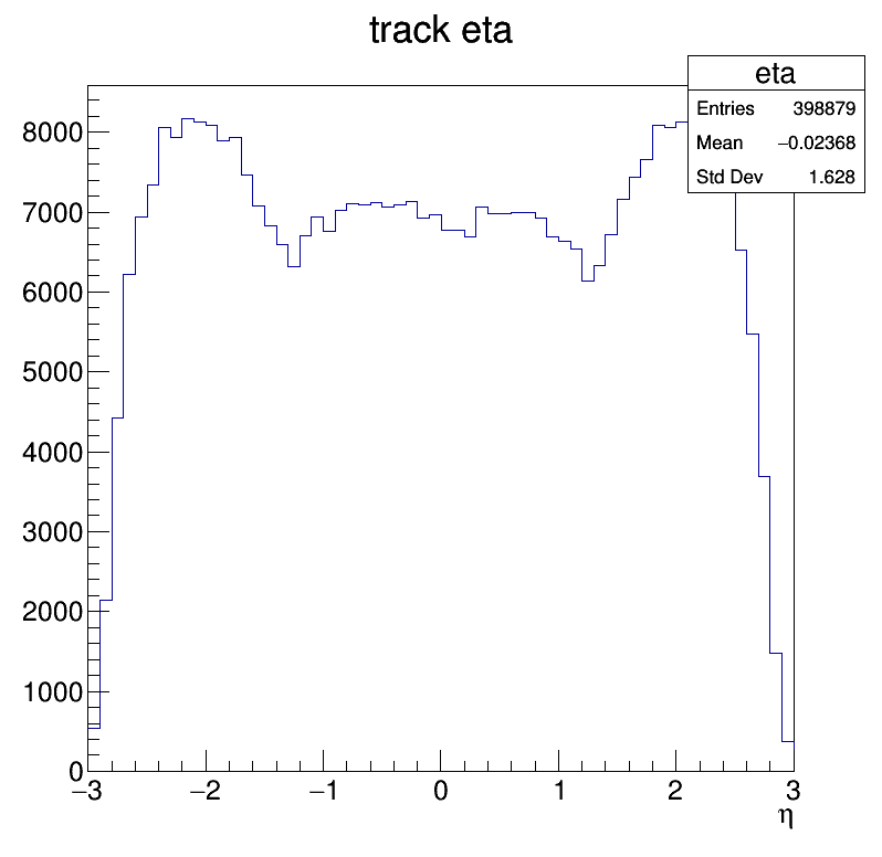
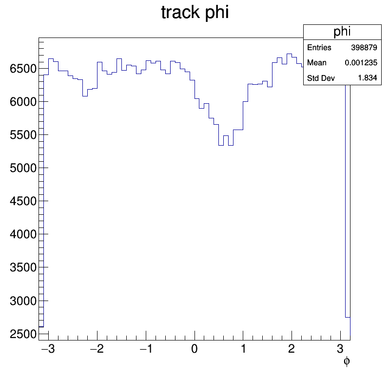
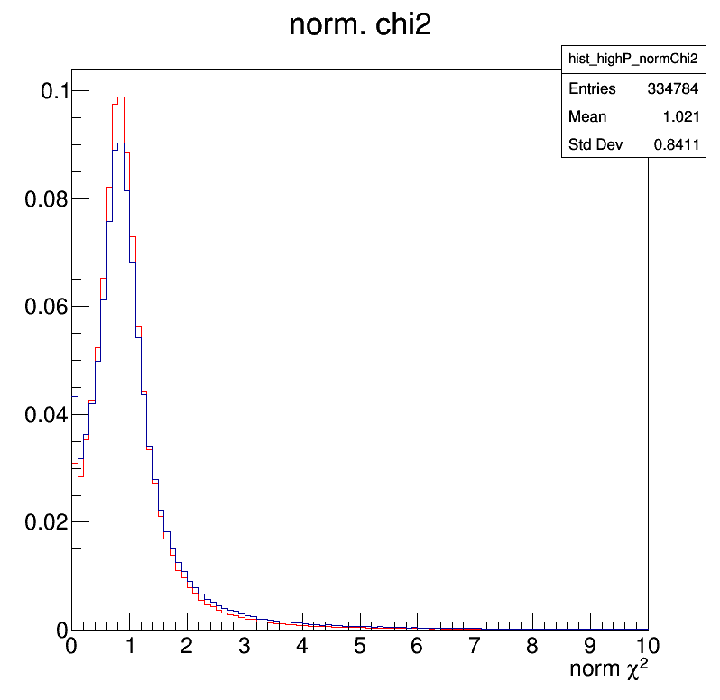
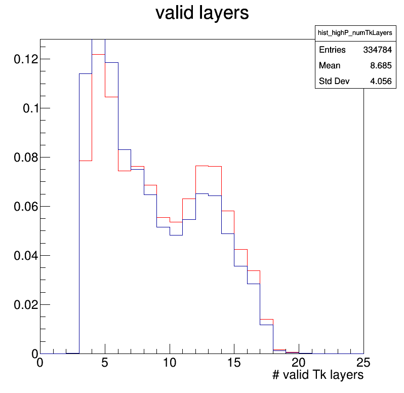
Now prepare plots for the track variables discussed above, as in the example below (name this file plot_track_quantities.py and put it in TrackingShortExercize/). Compare the distributions of track-quality-related variables (number of pixel hits, track goodness of fit, …, which are given in input to MVA classifiers) between tracks passing the highPurity and Loose quality flags. Do these distributions make sense to you?

Answer

import DataFormats.FWLite as fwlite
import ROOT

events = fwlite.Events("/eos/user/c/cmsdas/2023/short-ex-trk/run321167_ZeroBias_AOD.root")
tracks = fwlite.Handle("std::vector<reco::Track>")

hist_pt       = ROOT.TH1F("pt",       "track pt; p_{T} [GeV]", 100, 0.0, 100.0)
hist_eta      = ROOT.TH1F("eta",      "track eta; #eta", 60, -3.0, 3.0)
hist_phi      = ROOT.TH1F("phi",      "track phi; #phi", 64, -3.2, 3.2)

hist_loose_normChi2     = ROOT.TH1F("hist_loose_normChi2"    , "norm. chi2; norm #chi^{2}"        , 100, 0.0, 10.0)
hist_loose_numPixelHits = ROOT.TH1F("hist_loose_numPixelHits", "pixel hits; # pixel hits"         , 15, 0.0, 15.0)
hist_loose_numValidHits = ROOT.TH1F("hist_loose_numValidHits", "valid hits; # valid hits"         , 35, 0.0, 35.0)
hist_loose_numTkLayers  = ROOT.TH1F("hist_loose_numTkLayers" , "valid layers; # valid Tk layers"  , 25, 0.0, 25.0)
hist_highP_normChi2     = ROOT.TH1F("hist_highP_normChi2"    , "norm. chi2; norm #chi^{2}"        , 100, 0.0, 10.0)
hist_highP_numPixelHits = ROOT.TH1F("hist_highP_numPixelHits", "pixel hits; # pixel hits"         , 15, 0.0, 15.0)
hist_highP_numValidHits = ROOT.TH1F("hist_highP_numValidHits", "valid hits; # valid hits"         , 35, 0.0, 35.0)
hist_highP_numTkLayers  = ROOT.TH1F("hist_highP_numTkLayers" , "valid layers; # valid Tk layers"  , 25, 0.0, 25.0)

hist_highP_normChi2.SetLineColor(ROOT.kRed)
hist_highP_numPixelHits.SetLineColor(ROOT.kRed)
hist_highP_numValidHits.SetLineColor(ROOT.kRed)
hist_highP_numTkLayers.SetLineColor(ROOT.kRed)

for i, event in enumerate(events):
    event.getByLabel("generalTracks", tracks)
    for track in tracks.product():
        hist_pt.Fill(track.pt())
        hist_eta.Fill(track.eta())
        hist_phi.Fill(track.phi())

        if track.quality(track.qualityByName("loose")):
            hist_loose_normChi2    .Fill(track.normalizedChi2())
            hist_loose_numPixelHits.Fill(track.hitPattern().numberOfValidPixelHits())
            hist_loose_numValidHits.Fill(track.hitPattern().numberOfValidHits())
            hist_loose_numTkLayers .Fill(track.hitPattern().trackerLayersWithMeasurement())
        if track.quality(track.qualityByName("highPurity")):
            hist_highP_normChi2    .Fill(track.normalizedChi2())
            hist_highP_numPixelHits.Fill(track.hitPattern().numberOfValidPixelHits())
            hist_highP_numValidHits.Fill(track.hitPattern().numberOfValidHits())
            hist_highP_numTkLayers .Fill(track.hitPattern().trackerLayersWithMeasurement())

    if i > 500: break

c = ROOT.TCanvas( "c", "c", 800, 800)

hist_pt.Draw()
c.SetLogy()
c.SaveAs("track_pt.png")
c.SetLogy(False)

hist_eta.Draw()
c.SaveAs("track_eta.png")
hist_phi.Draw()
c.SaveAs("track_phi.png")

hist_highP_normChi2.DrawNormalized()
hist_loose_normChi2.DrawNormalized('same')
c.SaveAs("track_normChi2.png")
hist_highP_numPixelHits.DrawNormalized()
hist_loose_numPixelHits.DrawNormalized('same')
c.SaveAs("track_nPixelHits.png")
hist_highP_numValidHits.DrawNormalized()
hist_loose_numValidHits.DrawNormalized('same')
c.SaveAs("track_nValHits.png")
hist_highP_numTkLayers.DrawNormalized()
hist_loose_numTkLayers.DrawNormalized('same')
c.SaveAs("track_nTkLayers.png")

track_pt.png:
track_eta.png:
track_phi.png:
track_normChi2.png:
track_nPixelHits.png:
track_nTkLayers.png:
track_nValHits.png:

Track information in MiniAOD

There is no track collection stored in MiniAOD analogous to the generalTracks in AOD. Tracks associated to charged Particle Flow CandidatesPFCandidates are accessible directly from the packedPFCandidates collection for tracks with p_T > 0.5 GeV. For tracks between 0.5 and 0.95 GeV the track information is stored with reduced precision. Tracks not associated with PF candidates are in the lostTracks collection if their p_T is above 0.95 GeV or they are associated with a secondary vertex or a K_S or Lambda candidate. However, for both the tracks associated to the PFCandidates and the lostTracks, the highQuality track selection is used. Tracks with lower quality are not available in MiniAOD at all. In addition, tracks in the lostTracks collection are required to have at least 8 hits of which at least one has to be a pixel hit.

In particular, the track information saved in the PFCandidates is the following:

Track information in PFCandidates collection

the uncertainty on the impact parameter dzError(), dxyError()

the number of layers with hits on the track

the sub/det and layer of first hit of the track

the reco::Track of the candidate is provided by the pseudoTrack() method, with the following information stored:

the p_T,eta and phi of the original track (if those are different from the one of the original PFCandidate)

an approximate covariance matrix of the track state at the vertex

approximate hitPattern() and trackerExpectedHitsInner() that yield the correct number of hits, pixel hits, layers and the information returned by lostInnerHits()

the track normalized chisquare (truncated to an integer)

the highPurity quality flag set, if the original track had it.

Consider that the packedPFCandidates collects both charged and neutral candidates, therefore before trying to access the track information it is important to ensure that the candidate is charged and has the track information correctly stored (track.hasTrackDetails()).

Question 2

Write a simple script print-comparison.py that reads a MiniAOD file and the AOD file and compare plots of the same variables we looked at before for HighPurity tracks. For the track p_T distributuon, focus on the low p_T region below 5 GeV. Can you see any (non-statistical) difference with the previosu plots? You can copy a MiniAOD file with
cp /eos/user/c/cmsdas/2023/short-ex-trk/run321167_ZeroBias_MINIAOD.root $TMPDIR

Answer

import DataFormats.FWLite as fwlite
import ROOT
ROOT.gROOT.SetBatch(True)

events = fwlite.Events("/eos/user/c/cmsdas/2023/short-ex-trk/run321167_ZeroBias_MINIAOD.root")
eventsAOD = fwlite.Events("/eos/user/c/cmsdas/2023/short-ex-trk/run321167_ZeroBias_AOD.root")

tracks     = fwlite.Handle("std::vector<pat::PackedCandidate>")
losttracks = fwlite.Handle("std::vector<pat::PackedCandidate>")
tracksAOD = fwlite.Handle("std::vector<reco::Track>")

hist_pt       = ROOT.TH1F("pt",       "track pt; p_{T} [GeV]", 100, 0.0, 100.0)
hist_lowPt       = ROOT.TH1F("lowPt",       "track pt; p_{T} [GeV]", 100, 0.0, 5.0)
hist_eta      = ROOT.TH1F("eta",      "track eta; #eta", 60, -3.0, 3.0)
hist_phi      = ROOT.TH1F("phi",      "track phi; #phi", 64, -3.2, 3.2)

hist_normChi2     = ROOT.TH1F("hist_normChi2"    , "norm. chi2; norm #chi^{2}"        , 100, 0.0, 10.0)
hist_numPixelHits = ROOT.TH1F("hist_numPixelHits", "pixel hits; # pixel hits"         , 15, -0.5, 14.5)
hist_numValidHits = ROOT.TH1F("hist_numValidHits", "valid hits; # valid hits"         , 35, -0.5, 34.5)
hist_numTkLayers  = ROOT.TH1F("hist_numTkLayers" , "valid layers; # valid Tk layers"  , 25, -0.5, 24.5)

hist_pt_AOD       = ROOT.TH1F("ptAOD",       "track pt; p_{T} [GeV]", 100, 0.0, 100.0)
hist_lowPt_AOD    = ROOT.TH1F("lowPtAOD",       "track pt; p_{T} [GeV]", 100, 0.0, 5.0)
hist_eta_AOD      = ROOT.TH1F("etaAOD",      "track eta; #eta", 60, -3.0, 3.0)
hist_phi_AOD      = ROOT.TH1F("phiAOD",      "track phi; #phi", 64, -3.2, 3.2)

hist_normChi2_AOD     = ROOT.TH1F("hist_normChi2AOD"    , "norm. chi2; norm #chi^{2}"        , 100, 0.0, 10.0)
hist_numPixelHits_AOD = ROOT.TH1F("hist_numPixelHitsAOD", "pixel hits; # pixel hits"         , 15, -0.5, 14.5)
hist_numValidHits_AOD = ROOT.TH1F("hist_numValidHitsAOD", "valid hits; # valid hits"         , 35, -0.5, 34.5)
hist_numTkLayers_AOD  = ROOT.TH1F("hist_numTkLayersAOD" , "valid layers; # valid Tk layers"  , 25, -0.5, 24.5)

hist_pt_AOD.SetLineColor(ROOT.kRed)
hist_lowPt_AOD.SetLineColor(ROOT.kRed)
hist_eta_AOD.SetLineColor(ROOT.kRed)
hist_phi_AOD.SetLineColor(ROOT.kRed)

hist_normChi2_AOD.SetLineColor(ROOT.kRed)
hist_numPixelHits_AOD.SetLineColor(ROOT.kRed)
hist_numValidHits_AOD.SetLineColor(ROOT.kRed)
hist_numTkLayers_AOD.SetLineColor(ROOT.kRed)

for i, event in enumerate(events):
    event.getByLabel("packedPFCandidates", "", tracks)
    event.getByLabel("lostTracks", "", losttracks)

    alltracks  = [track for track in tracks.product()]
    alltracks += [track for track in losttracks.product()]

    for track in alltracks :
        if (not track.hasTrackDetails() or track.charge() == 0 ):
            continue
        if not track.trackHighPurity():
            continue
        hist_pt.Fill(track.pt())
        hist_lowPt.Fill(track.pt())
        hist_eta.Fill(track.eta())
        hist_phi.Fill(track.phi())

        hist_normChi2    .Fill(track.pseudoTrack().normalizedChi2())
        hist_numPixelHits.Fill(track.numberOfPixelHits())
        hist_numValidHits.Fill(track.pseudoTrack().hitPattern().numberOfValidHits())
        hist_numTkLayers .Fill(track.pseudoTrack().hitPattern().trackerLayersWithMeasurement())

    if i > 1000: break

for i, event in enumerate(eventsAOD):
    event.getByLabel("generalTracks", tracksAOD)

    for j, track in enumerate(tracksAOD.product()) :
        if not track.quality(track.qualityByName("highPurity")):
            continue

        hist_pt_AOD.Fill(track.pt())
        hist_lowPt_AOD.Fill(track.pt())
        hist_eta_AOD.Fill(track.eta())
        hist_phi_AOD.Fill(track.phi())

        hist_normChi2_AOD    .Fill(track.normalizedChi2())
        hist_numPixelHits_AOD.Fill(track.hitPattern().numberOfValidPixelHits())
        hist_numValidHits_AOD.Fill(track.hitPattern().numberOfValidHits())
        hist_numTkLayers_AOD .Fill(track.hitPattern().trackerLayersWithMeasurement())

    if i > 1000: break

c = ROOT.TCanvas( "c", "c", 800, 800)

hist_pt.Draw()
hist_pt_AOD.Draw("same")
c.SetLogy()
c.SaveAs("track_pt_miniaod.png")

hist_lowPt_AOD.Draw()
hist_lowPt.Draw("same")
c.SetLogy()
c.SaveAs("track_lowPt_miniaod.png")
c.SetLogy(False)
hist_eta_AOD.Draw()
hist_eta.Draw("same")
c.SaveAs("track_eta_miniaod.png")
hist_phi_AOD.Draw()
hist_phi.Draw("same")
c.SaveAs("track_phi_miniaod.png")

hist_normChi2_AOD.Draw()
hist_normChi2.Draw("same")
c.SaveAs("track_normChi2_miniaod.png")
hist_numPixelHits_AOD.Draw()
hist_numPixelHits.Draw("same")
c.SaveAs("track_nPixelHits_miniaod.png")
hist_numValidHits_AOD.Draw()
hist_numValidHits.Draw("same")
c.SaveAs("track_nValHits_miniaod.png")
hist_numTkLayers_AOD.Draw()
hist_numTkLayers.Draw("same")
c.SaveAs("track_nTkLayers_miniaod.png")

Key Points

The pre-selection of tracks to HighPurity in MiniAOD also affects the distribution of the track quality parameters.

All tracks are stored in the generalTracks collection in AOD.

In MiniAOD they are accessible in a less straightforward way (packedPFCandidates, lostTracks collection) and not all tracks are available!

CMS Data Analysis School Tracking and Vertexing Short Exercise - Tracks as particles

Overview

Teaching: 10 min
Exercises: 10 min

Questions

Can we consider a track as a particle?

Can I use an alternative to the muon object?

Can I define the invariant mass of two tracks?

Objectives

Being familiar with the tracks, particle and identification concepts.

Plot distributions of variables related to a muon resonance.

Unlike calorimeter showers, tracks can usually be interpreted as particle 4-vectors without any additional corrections. Detector alignment, non-helical trajectories from energy loss, Lorentz angle corrections, and (to a much smaller extent) magnetic field inhomogeneities are important, but they are all corrections that must be applied during or before the track-reconstruction process. From an analyzer’s point of view, most tracks are individual particles (depending on quality cuts) and the origin and momentum of the particle are derived from the track’s geometry, with some resolution (random error). Biases (systematic offsets from the true values) are not normal: they’re an indication that something went wrong in this process. The analyzer does not even need to calculate the particle’s momentum from the track parameters: there are member functions for that. Particle’s transverse momentum, momentum magnitude, and all of its components can be read through the following lines (let’s name this new file kinematics.py and create it in TrackingShortExercize/):

import DataFormats.FWLite as fwlite
import ROOT
import math

events = fwlite.Events("/eos/user/c/cmsdas/2023/short-ex-trk/run321167_ZeroBias_AOD.root")
tracks = fwlite.Handle("std::vector<reco::Track>")

for i, event in enumerate(events):
    event.getByLabel("generalTracks", tracks)
    for track in tracks.product():
        print track.pt(), track.p(), track.px(), track.py(), track.pz()
    if i > 20: break

Question 1

Now we can use this to do some kinematics. Assuming that the particle is a pion (pion mass = 0.140 GeV), calculate its kinetic energy.

Answer

import DataFormats.FWLite as fwlite
import ROOT
import math

events = fwlite.Events("/eos/user/c/cmsdas/2023/short-ex-trk/run321167_ZeroBias_AOD.root")
tracks = fwlite.Handle("std::vector<reco::Track>")

for i, event in enumerate(events):
    event.getByLabel("generalTracks", tracks)
    for track in tracks.product():
        print track.pt(), track.p(), track.px(), track.py(), track.pz()
        print "energy: ", math.sqrt(0.140**2 + track.p()**2)
    if i > 20: break

Additional information

Identifying the particle that made the track is difficult: the mass of some low-momentum tracks can be identified by their energy loss, called dE/dx, and electrons and muons can be identified by signatures in other subdetectors. Without any other information, the safest assumption is that a randomly chosen track is a pion, since hadron collisions produce a lot of pions.

Let’s look for resonances. Given two tracks,

if len(tracks.product()) > 1:

one = tracks.product()[0]
two = tracks.product()[1]

the invariant mass may be calculated as

total_energy = math.sqrt(0.140**2 + one.p()**2) + math.sqrt(0.140**2 + two.p()**2)
total_px = one.px() + two.px()
total_py = one.py() + two.py()
total_pz = one.pz() + two.pz()
mass = math.sqrt(total_energy**2 - total_px**2 - total_py**2 - total_pz**2)

However, this quantity has no meaning unless the two particles are actually descendants of the same decay. Two randomly chosen tracks (out of hundreds per event) typically are not.

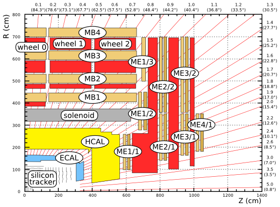
To increase the chances that pairs of randomly chosen tracks are descendants of the same decay, consider a smaller set of tracks: muons. Muons are identified by the fact that they can pass through meters of iron (the CMS magnet return yoke), so muon tracks extend from the silicon tracker to the muon chambers (see CMS quarter-view below), as much as 12 meters long! Muons are rare in hadron collisions. If an event contains two muons, they often (though not always) come from the same decay.

Normally, one would access muons through the reco::Muon object since this contains additional information about the quality of the muon hypothesis. For simplicity, we will access their track collection in the same way that we have been accessing the main track collection. We only need to replace generalTracks with globalMuons. Add the following loop to kinematics.py.

events.toBegin()
for i, event in enumerate(events):
    if i >= 15: break            # only the first 15 events
    print "Event", i
    event.getByLabel("globalMuons", tracks)
    for j, track in enumerate(tracks.product()):
        print "    Track", j, track.charge()/track.pt(), track.phi(), track.eta(), track.dxy(), track.dz()

Run this code on the run321167_Charmonium_AOD.root file that you can copy with:

cp /eos/user/c/cmsdas/2023/short-ex-trk/run321167_Charmonium_AOD.root $TMPDIR

Notice how few muon tracks there are compared to the same code executed for generalTracks. In fact, you only see as many muons as you do because this data sample was collected with a muon trigger. (The muon definition in the trigger is looser than the globalMuons algorithm, which is why there are some events with fewer than two globalMuons.) See in the Appendix an application for the Muon and Tracks objects usage in the CMS tracking efficiency computation.

Question 2

As an exercise, make a histogram of all di-muon masses from 0 to 5 GeV. Exclude events that do not have exactly two muon tracks, and note that the muon mass is 0.106 GeV). Create a file dimuon_mass.py in TrackingShortExercize/ for this purpose.

More…

The solution combines several of the techniques introduced above:

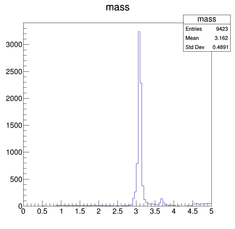
import math
import DataFormats.FWLite as fwlite
import ROOT

events = fwlite.Events("/eos/user/c/cmsdas/2023/short-ex-trk/run321167_Charmonium_AOD.root")
tracks = fwlite.Handle("std::vector<reco::Track>")
mass_histogram = ROOT.TH1F("mass", "mass", 100, 0.0, 5.0)

events.toBegin()
for event in events:
    event.getByLabel("globalMuons", tracks)
    product = tracks.product()
    if product.size() == 2:
        one = product[0]
        two = product[1]
        if not (one.charge()*two.charge() == -1):  continue
        energy = (math.sqrt(0.106**2 + one.p()**2) +
                  math.sqrt(0.106**2 + two.p()**2))
        px = one.px() + two.px()
        py = one.py() + two.py()
        pz = one.pz() + two.pz()
        mass = math.sqrt(energy**2 - px**2 - py**2 - pz**2)
        mass_histogram.Fill(mass)

c = ROOT.TCanvas ("c", "c", 800, 800)
mass_histogram.Draw()
c.SaveAs("mass.png")

The histogram should look like this:

If so, congratulations! You’ve discovered the J/ψ!

Key Points

Tracks give us a direct handle on actual particles, thus they can easily be used to reconstruct other particles in the event

CMS Data Analysis School Tracking and Vertexing Short Exercise - Constructing vertices from tracks

Overview

Teaching: 20 min
Exercises: 20 min

Questions

What is a (primary, secondary) vertex object? What about beamspot?

Which information are available in different CMS data formats?

How can I run the vertex reconstruction?

Can we get better physics results using primary verteces?

Objectives

Being familiar with the vertex concept.

Plot distributions about the main vertex variables.

Open the stage for Appendix exercises.

In this exercise, we will encounter three main objects: primary vertices, secondary vertices, and the beamspot. Let’s start with secondary vertices. Particles produced by a single decay or collision radiate from the point of their origin. Their tracks should nearly cross at this point (within measurement uncertainties): if two or more tracks cross at some point, it is very likely that they descend from the same decay or collision.

This test is more significant than it may appear by looking at event pictures. With so many tracks, it looks like they cross accidentally, but the two-dimensional projection of the event picture is misleading. One-dimensional paths through three-dimensional space do not intersect easily, especially when the trajectories of those paths are measured with microns to hundreds-of-microns precision.

Starting from the detected tracks, we work backward and reconstruct the original vertices by checking each pair of tracks for overlaps. This is performed in the standard reconstruction sequence and delivered to the analyst as lists of K_S → π⁺π^- and Λ → pπ⁰ candidates, but we will repeat the procedure with different parameters. The algorithm will run three times, the first accepting all (loose) tracks, the second accepting only tight tracks, and the third accepting only highPurity tracks.

These are called secondary vertices because the proton-proton collision produced the first (primary) vertex, then the neutral K_S flew several centimeters away from the rest of the collision products and decayed into π⁺π^- at a second (secondary) position in space.

Running the vertex reconstruction

Create a file named construct_secondary_vertices_cfg.py in TrackingShortExercize/ and fill it with the following:

import FWCore.ParameterSet.Config as cms

process = cms.Process("KSHORTS")

# Use the tracks_and_vertices.root file as input.
process.source = cms.Source("PoolSource",
    fileNames = cms.untracked.vstring("file:/eos/user/c/cmsdas/2023/short-ex-trk/run321167_Charmonium_AOD.root"))
process.maxEvents = cms.untracked.PSet(input = cms.untracked.int32(500))

# Suppress messages that are less important than ERRORs.
process.MessageLogger = cms.Service("MessageLogger",
    destinations = cms.untracked.vstring("cout"),
    cout = cms.untracked.PSet(threshold = cms.untracked.string("ERROR")))

# Load part of the CMSSW reconstruction sequence to make vertexing possible.
# We'll need the CMS geometry and magnetic field to follow the true, non-helical
# shapes of tracks through the detector.
process.load("Configuration/StandardSequences/FrontierConditions_GlobalTag_cff")
from Configuration.AlCa.GlobalTag import GlobalTag
process.GlobalTag =  GlobalTag(process.GlobalTag, "auto:run2_data")
process.load("Configuration.Geometry.GeometryRecoDB_cff")
process.load("Configuration.StandardSequences.MagneticField_cff")
process.load("TrackingTools.TransientTrack.TransientTrackBuilder_cfi")

# Copy most of the vertex producer's parameters, but accept tracks with
# progressively more strict quality.
process.load("RecoVertex.V0Producer.generalV0Candidates_cfi")

# loose
process.SecondaryVerticesFromLooseTracks = process.generalV0Candidates.clone(
    trackRecoAlgorithm = cms.InputTag("generalTracks"),
    doKshorts = cms.bool(True),
    doLambdas = cms.bool(True),
    trackQualities = cms.string("loose"),
    innerHitPosCut = cms.double(-1.),
    cosThetaXYCut = cms.double(-1.), 
    )

# tight
process.SecondaryVerticesFromTightTracks = process.SecondaryVerticesFromLooseTracks.clone(
    trackQualities = cms.string("tight"),
    )

# highPurity
process.SecondaryVerticesFromHighPurityTracks = process.SecondaryVerticesFromLooseTracks.clone(
    trackQualities = cms.string("highPurity"),
    )

# Run all three versions of the algorithm.
process.path = cms.Path(process.SecondaryVerticesFromLooseTracks *
                        process.SecondaryVerticesFromTightTracks *
                        process.SecondaryVerticesFromHighPurityTracks)

# Writer to a new file called output.root.  Save only the new K-shorts and the
# primary vertices (for later exercises).
process.output = cms.OutputModule(
    "PoolOutputModule",
    SelectEvents = cms.untracked.PSet(SelectEvents = cms.vstring("path")),
    outputCommands = cms.untracked.vstring(
        "drop *",
        "keep *_*_*_KSHORTS",
        "keep *_offlineBeamSpot_*_*",
        "keep *_offlinePrimaryVertices_*_*",
        "keep *_offlinePrimaryVerticesWithBS_*_*",
        ),
    fileName = cms.untracked.string("output.root")
    )
process.endpath = cms.EndPath(process.output)

The name of the secondary-vertex producer (process.SecondaryVerticesFromLooseTracks) given in this configuration will be the name of the produced collection with process. stripped off (see the usage below). Run the configuration file with:

cmsRun construct_secondary_vertices_cfg.py

which can take a couple of minutes to complete. Notice it will create the output.root file which will be used later. You can check the content of the file by running the simple script as follows

edmDumpEventContent output.root

Looking at secondary vertices

When it’s done, you can open output.root and read the vertex positions, just as you did for the track momenta with the following lines (let’s name this code sec_vertices.py and put it in TrackingShortExercize/):

import DataFormats.FWLite as fwlite

events = fwlite.Events("file:output.root")
secondaryVertices = fwlite.Handle("std::vector<reco::VertexCompositeCandidate>")

events.toBegin()
for i, event in enumerate(events):
    print "Event:", i
    event.getByLabel("SecondaryVerticesFromLooseTracks", "Kshort", secondaryVertices)
    for j, vertex in enumerate(secondaryVertices.product()):
        print "    Vertex:", j, vertex.vx(), vertex.vy(), vertex.vz()
    if i > 10: break

In the code above, you specify the C++ type of the collection (std::vector). For each event you obtain the collection of secondary vertices originating from K_S decays, by providing the name of the collection producer (SecondaryVerticesFromLooseTracks) and the label for the K_S collection (Kshort, defined here).

Each of these vertices contains two tracks by construction. One of the vertex member functions (do dir(vertex) in the python shell after executing the above code to see them all) returns the invariant mass of the pair of tracks. This calculation is a little more complex than the invariant masses we calculated by hand because it is necessary to evaluate the px and py components of momentum at the vertex rather than at the beamspot. If these two particles really did originate in a decay several centimeters from the beamspot, then the track parameters evaluated at the beamspot are not meaningful.

Question 1

Plot the invariant mass of all vertices. Modify the sec_vertices.py to draw the invariant mass distribution, i.e. fill a histogram with vertex.mass() for each secondary vertex.

Answer (don’t look until you’ve tried it!)

import DataFormats.FWLite as fwlite
import ROOT

events = fwlite.Events("file:output.root")
secondaryVertices = fwlite.Handle("std::vector<reco::VertexCompositeCandidate>")

mass_histogram = ROOT.TH1F("mass", "mass", 100, 0.4, 0.6)

events.toBegin()
for event in events:
    event.getByLabel("SecondaryVerticesFromLooseTracks", "Kshort", secondaryVertices)
    for vertex in secondaryVertices.product():
        mass_histogram.Fill(vertex.mass())

c = ROOT.TCanvas ("c" , "c", 800, 800)
mass_histogram.Draw()
c.SaveAs("kshort_mass.png")

Question 2

You should see a very prominent K_S → π⁺π^- peak, but also a pedestal. What is the pedestal? Why does it cut off at 0.43 and 0.57 GeV?

More

You can answer the question concerning the cut-off with the information here.

Question 3

Prepare a similar plot for the Lambda vertices. (Hints: were the Lambda vertices created when you ran the SecondaryVertices producer? the Lambda mass is 1.115 GeV. Are you expecting to reconstruct the mass at the same value in the whole detector ? (optionally plot the mass resolution as function of the eta of the reconstructed Lambda).

Question 4

Plot the flight distance of all vertices. Modify the sec_vertices.py to draw the flight distance in the transverse plane distribution between each secondary vertex and the primary vertex (PV). For this, you can look ahead at the next part of the exercise to see how to access the primary vertices collection. Once you have it, you can access the first primary vertex in the collection with pv = primaryVertices.product()[0]. You can now use the x and y coordinates of the secondary vertices and the primary vertex to calculate the distance. Note that for the PV, you access these values with the x() and y() member functions, while for the secondary vertices, these are called vx() and vy().

Answer

import DataFormats.FWLite as fwlite
import ROOT

events = fwlite.Events("file:output.root")
secondaryVertices = fwlite.Handle("std::vector<reco::VertexCompositeCandidate>")
primaryVertices = fwlite.Handle("std::vector<reco::Vertex>")

lxy_histogram = ROOT.TH1F("lxy", "lxy", 500, 0, 70)

events.toBegin()
for event in events:
    event.getByLabel("offlinePrimaryVertices", primaryVertices)
    pv = primaryVertices.product()[0]
    event.getByLabel("SecondaryVerticesFromLooseTracks", "Lambda", secondaryVertices)
    for vertex in secondaryVertices.product():
        lxy = ((vertex.vx()-pv.x())**2 + (vertex.vy() - pv.y())**2)**0.5
        lxy_histogram.Fill(lxy)
c = ROOT.TCanvas ("c" , "c", 800, 800)
lxy_histogram.Draw()
c.SaveAs("lambda_lxy.png")

Question 5

You should rerun the construct_secondary_vertices.py to process all events in the file to get more statistics. For this, set the maxEvents parameter to -1. Running on more events, one can appreciate some structures in the flight distance distribution, can you explain them ? Note that these are especially noticeable in the distribution of Lambdas.

Secondary vertices in MiniAOD

The SecondaryVertex collection is already available in the MiniAOD files. You can retrieve the collection type and format by doing:

 cp /eos/user/c/cmsdas/2023/short-ex-trk/run321167_Charmonium_MINIAOD.root $TMPDIR
 edmDumpEventContent $TMPDIR/run321167_Charmonium_MINIAOD.root | grep Vertices

Question 6

Modify sec_vertices.py to read the lambda vertices from the MiniAOD file. You will have to modify the collection type and label accordingly to the MiniAOD content.

Answer

import DataFormats.FWLite as fwlite
import ROOT

events = fwlite.Events("/eos/user/c/cmsdas/2023/short-ex-trk/run321167_Charmonium_MINIAOD.root")
secondaryVertices = fwlite.Handle("std::vector<reco::VertexCompositePtrCandidate>")

mass_histogram = ROOT.TH1F("mass_histogram", "mass_histogram", 100, 1., 1.2)

events.toBegin()
for i, event in enumerate(events):
    event.getByLabel("slimmedLambdaVertices", "", secondaryVertices)
    for j, vertex in enumerate(secondaryVertices.product()):
        mass_histogram.Fill(vertex.mass())

c = ROOT.TCanvas()
mass_histogram.Draw()
c.SaveAs("mass_lambda_miniaod.png")

Basic distributions of primary vertices

The primary vertex reconstruction consists of three steps:

Steps of primary vertex reconstruction

Selection of tracks

Clustering of the tracks that appear to originate from the same interaction vertex

Fitting for the position of each vertex using its associated tracks

All the primary vertices reconstructed in an event are saved in the reco::Vertex collection labeled offlinePrimaryVertices. Create the file vertex.py in TrackingShortExercize/ which will load the original run321167_ZeroBias_AOD.root file and make a quarter-view plot of the vertex distribution (run it using python vertex.py):

import DataFormats.FWLite as fwlite
import math
import ROOT

events = fwlite.Events("/eos/user/c/cmsdas/2023/short-ex-trk/run321167_ZeroBias_AOD.root")
primaryVertices = fwlite.Handle("std::vector<reco::Vertex>")

rho_z_histogram = ROOT.TH2F("rho_z", "rho_z", 100, 0.0, 30.0, 100, 0.0, 10.0)

events.toBegin()
for event in events:
    event.getByLabel("offlinePrimaryVertices", primaryVertices)
    for vertex in primaryVertices.product():
        rho_z_histogram.Fill(abs(vertex.z()),
                             math.sqrt(vertex.x()**2 + vertex.y()**2))

c = ROOT.TCanvas("c", "c", 800, 800)
rho_z_histogram.Draw()
c.SaveAs("rho_z.png")

You should see a broad distribution in z, close to rho = 0 (much closer than for the secondary vertices, see appendix). In fact, the distribution is about 0.1 cm wide and 4 cm long. The broad distribution in z is helpful: if 20 primary vertices are uniformly distributed along a 4 cm pencil-like region, we only need 2 mm vertex resolution to distinguish neighboring vertices. Fortunately, the CMS vertex resolution is better than this (better than 20μm and 25μm in x and z, respectively TRK-11-001, performances with the Phase1 pixel detector), so they can be distinguished with high significance.

To see this, you should modify properly the previous code to make a plot of the distance between primary vertices:

deltaz_histogram = ROOT.TH1F("deltaz", "deltaz", 1000, -20.0, 20.0)

events.toBegin()
for event in events:
    event.getByLabel("offlinePrimaryVertices", primaryVertices)
    pv = primaryVertices.product()
    for i in xrange(pv.size() - 1):
        for j in xrange(i + 1, pv.size()):
            deltaz_histogram.Fill(pv[i].z() - pv[j].z())

c = ROOT.TCanvas ("c", "c", 800, 800)
deltaz_histogram.Draw()
c.SaveAs("deltaz.png")

The broad distribution is due to the spread in primary vertex positions. Zoom in on the narrow dip near deltaz = 0. This region is empty because if two real vertices are too close to each other, they will be misreconstructed as a single vertex. Thus, there are no reconstructed vertices with such small separations.

Question 7

Write a short script to print out the number of primary vertices in each event. When people talk about the pile-up, it is this number they are referring to. If you want, you can even plot it; the distribution should roughly fit a Poisson distribution.

Answer

events.toBegin()
for i, event in enumerate(events):
    event.getByLabel("offlinePrimaryVertices", primaryVertices)
    print "Pile-up:", primaryVertices.product().size()
    if i > 100: break

Print out the number of tracks in a single vertex object. (Use the trick for vertex in primaryVertices.product(): break to obtain a primary vertex object.)

Solution
print vertex.nTracks()
print vertex.tracksSize()
Why might they be different? ( See tracksSize vs nTracks). Note: in C++, you could loop over the tracks associated with this vertex, but this functionality doesn’t work in Python. In the standard analysis workflow there are many quality requirements to be applied to the events and to the reconstructed quantities in an event. One of these requests is based on the characteristics of the reconstructed primary vertices, and it is defined by the CMSSW EDFilter goodOfflinePrimaryVertices_cfi.py . Are these selections surprising you ?

Question 8

Write a short script to plot the distribution of the number of tracks vs the number of vertices. What do you expect?

Answer

The following snippet tells you what to do, but you need to make sure that all needed variables are defined.

histogram = ROOT.TH2F("ntracks_vs_nvertex","ntracks_vs_nvertex",
                      30, 0.0, 29.0, 100, 0.0,2000.0)

events.toBegin()
for event in events:
    event.getByLabel("offlinePrimaryVertices", primaryVertices)
    event.getByLabel("generalTracks", tracks)
    histogram.Fill(primaryVertices.product().size(), tracks.product().size())

c = ROOT.TCanvas("c", "c", 800, 800)
histogram.Draw()
c.SaveAs("ntracks_vs_nvertex.png")

It’s also useful to distinguish between the primary vertices and the beamspot. A read-out event can have many primary vertices, each of which usually corresponds to a point in space where two protons collide. The beamspot is an estimate of where protons are expected to collide, derived from the distribution of primary vertices. Not only does an event have only one beamspot, but the beamspot is constant for a lumi-section (time interval of 23.31 consecutive seconds). This script prints the average x-position of the primary vertices and plots their x-y distribution (name it beamspot.py and put it in TrackingShortExercize):

import DataFormats.FWLite as fwlite
import math
import ROOT

def isGoodPV(vertex):
    if ( vertex.isFake()        or 
         vertex.ndof < 4.0      or 
         abs(vertex.z()) > 24.0 or 
         abs(vertex.position().Rho()) > 2):
           return False
    return True

events          = fwlite.Events("/eos/user/c/cmsdas/2023/short-ex-trk/run321167_ZeroBias_AOD.root")
primaryVertices = fwlite.Handle("std::vector<reco::Vertex>")
beamspot        = fwlite.Handle("reco::BeamSpot")

vtx_xy = ROOT.TH2F('vtx_xy','; x [cm]; y [cm]', 100,-0.1, 0.3, 100, -0.25, 0.15)

sumx = 0.0
N    = 0
last_beamspot = None

events.toBegin()
for event in events:
    event.getByLabel("offlinePrimaryVertices", primaryVertices)
    event.getByLabel("offlineBeamSpot", beamspot)

    if last_beamspot == None or last_beamspot != beamspot.product().x0():
        print "New beamspot IOV (interval of validity)..."
        last_beamspot       = beamspot.product().x0()
        sumx = 0.0
        N = 0

    for vertex in primaryVertices.product():
        if not isGoodPV(vertex):  continue
        N += 1
        sumx += vertex.x()
        vtx_xy.Fill(vertex.x(), vertex.y())
        if N % 1000 == 0:
            print "Mean of primary vertices:", sumx/N,
            print "Beamspot:", beamspot.product().x0()
            
c = ROOT.TCanvas( "c", "c", 1200, 800)
vtx_xy.Draw("colz")
c.SaveAs("vtx_xy.png")

Add the analogous 2D plots for x versus z and y vs z positions.

More exercises…

Furthermore, you can add a plot of the average primary vertex position and compare it to:

the center of beamspot (red line)

the beamspot region (beamspot center +/- beamspot witdh, that you can access through beamspot.product().BeamWidthX()

Answer

import DataFormats.FWLite as fwlite
import math
import ROOT
from array import array

ROOT.gROOT.SetBatch(True)

def isGoodPV(vertex):
    if ( vertex.isFake()        or \
         vertex.ndof < 4.0      or \
         abs(vertex.z()) > 24.0 or \
         abs(vertex.position().Rho()) > 2):
           return False
    return True

events          = fwlite.Events("/eos/user/c/cmsdas/2023/short-ex-trk/run321167_ZeroBias_AOD.root")
primaryVertices = fwlite.Handle("std::vector<reco::Vertex>")
beamspot        = fwlite.Handle("reco::BeamSpot")
vtx_position, N_vtx = array( 'd' ), array( 'd' )

vtx_xy = ROOT.TH2F('vtx_xy','; x [cm]; y [cm]', 100,-0.05, 0.25, 100, -0.2, 0.1)
c = ROOT.TCanvas( "c", "c", 1200, 800)

sumx = 0.0
N    = 0
iIOV = 0
last_beamspot = None
last_beamspot_sigma = None

vtx_position, N_vtx = array( 'd' ), array( 'd' )
leg = ROOT.TLegend(0.45, 0.15, 0.6, 0.28)
leg.SetBorderSize(0)
leg.SetTextSize(0.03)

events.toBegin()
for event in events:
    event.getByLabel("offlinePrimaryVertices", primaryVertices)
    event.getByLabel("offlineBeamSpot", beamspot)

    if last_beamspot == None or last_beamspot != beamspot.product().x0():
        print "New beamspot IOV (interval of validity)..."

        ## first save tgraph and then reset
        if (iIOV > 0):
            theGraph   = ROOT.TGraph(len(vtx_position), N_vtx, vtx_position)
            theGraph.SetMarkerStyle(8)
            theGraph.SetTitle('IOV %s; N Vtx; X position'%iIOV)
            theGraph.Draw('AP')
            theGraph.GetYaxis().SetRangeUser(0.094, 0.100)
            
            line = ROOT.TLine(0,last_beamspot,N_vtx[-1],last_beamspot)
            line.SetLineColor(ROOT.kRed)
            line.SetLineWidth(2)
            line.Draw()

            line2 = ROOT.TLine(0,last_beamspot - last_beamspot_sigma,N_vtx[-1],last_beamspot - last_beamspot_sigma)
            line2.SetLineColor(ROOT.kOrange)
            line3 = ROOT.TLine(0,last_beamspot + last_beamspot_sigma,N_vtx[-1],last_beamspot + last_beamspot_sigma)
            line3.SetLineColor(ROOT.kOrange)
            line2.SetLineWidth(2)
            line3.SetLineWidth(2)
            line2.Draw()
            line3.Draw()
            
            leg.Clear()
            leg.AddEntry(theGraph,  'ave. vtx position',        'p')
            leg.AddEntry(line    ,  'center of the beamspot ' , 'l')
            leg.AddEntry(line2   ,  'center of the bs #pm beamspot width ' , 'l')
            leg.Draw()
            c.SaveAs("vtx_x_vs_N_%s.png"%iIOV)
            break

            vtx_position, N_vtx = array( 'd' ), array( 'd' )

        last_beamspot       = beamspot.product().x0()
        last_beamspot_sigma = beamspot.product().BeamWidthX()
        sumx = 0.0
        N = 0
        iIOV += 1

    for vertex in primaryVertices.product():
        if not isGoodPV(vertex):  continue
        N += 1
        sumx += vertex.x()
        if N % 1000 == 0:
            vtx_position.append(sumx/N)
            N_vtx.append(N)

Primary vertices improve physics results

Finally, let’s consider an example of how primary vertices are useful to an analyst. If you’re interested in K_S → π⁺π^-, it might seem that primary vertices are irrelevant because neither of your two visible tracks (π⁺π^-) directly originated in any of the proton-proton collisions. However, the K_S did. The K_S flew several centimeters away from the primary vertex in which it was produced, and its direction of flight must be parallel to its momentum (by definition).

We can measure the K_S momentum from the momenta of its decay products, and we can identify the start and end positions of the K_S flight from the locations of the primary and secondary vertices. The momentum vector and the displacement vector must be parallel. (There is no constraint on the length of the displacement vector because the lifetimes of K_S mesons follow an exponentially random distribution.)

Create a new file analyse.py in TrackingShortExercize/ which will open output.root:

import math
import DataFormats.FWLite as fwlite
import ROOT

events = fwlite.Events("file:output.root")
primaryVertices = fwlite.Handle("std::vector<reco::Vertex>")
secondaryVertices = fwlite.Handle("std::vector<reco::VertexCompositeCandidate>")

Create a histogram in which to plot the distribution of cosAngle, which is the normalized dot product of the K_S momentum vector and its displacement vector. Actually, make two histograms to zoom into the cosAngle → 1 region.

cosAngle_histogram = ROOT.TH1F("cosAngle", "cosAngle", 100, -1.0, 1.0)
cosAngle_zoom_histogram = ROOT.TH1F("cosAngle_zoom", "cosAngle_zoom", 100, 0.99, 1.0)

Question 9

Construct a nested loop over secondary and primary vertices to compute displacement vectors and compare them with K_S momentum vectors. Just print out a few values.

Answer

for i, event in enumerate(events):
    event.getByLabel("offlinePrimaryVertices", primaryVertices)
    event.getByLabel("SecondaryVerticesFromLooseTracks", "Kshort", secondaryVertices)
    for secondary in secondaryVertices.product():
        px = secondary.px()
        py = secondary.py()
        pz = secondary.pz()
        p = secondary.p()
        for primary in primaryVertices.product():
            dx = secondary.vx() - primary.x()
            dy = secondary.vy() - primary.y()
            dz = secondary.vz() - primary.z()
            dl = math.sqrt(dx**2 + dy**2 + dz**2)
            print "Normalized momentum:", px/p, py/p, pz/p,
            print "Normalized displacement:", dx/dl, dy/dl, dz/dl
    if i > 20: break

For each set of primary vertices, find the best cosAngle and fill the histograms with that.

Solution

import math
import DataFormats.FWLite as fwlite
import ROOT

events = fwlite.Events("file:output.root")
primaryVertices = fwlite.Handle("std::vector<reco::Vertex>")
secondaryVertices = fwlite.Handle("std::vector<reco::VertexCompositeCandidate>")

cosAngle_histogram = ROOT.TH1F("cosAngle", "cosAngle", 100, -1.0, 1.0)
cosAngle_zoom_histogram = ROOT.TH1F("cosAngle_zoom", "cosAngle_zoom", 100, 0.99, 1.0)

events.toBegin()
for event in events:
    event.getByLabel("offlinePrimaryVertices", primaryVertices)
    event.getByLabel("SecondaryVerticesFromLooseTracks", "Kshort", secondaryVertices)
    for secondary in secondaryVertices.product():
        px = secondary.px()
        py = secondary.py()
        pz = secondary.pz()
        p = secondary.p()
        bestCosAngle = -1       # start with the worst possible
        for primary in primaryVertices.product():
            dx = secondary.vx() - primary.x()
            dy = secondary.vy() - primary.y()
            dz = secondary.vz() - primary.z()
            dl = math.sqrt(dx**2 + dy**2 + dz**2)
            dotProduct = px*dx + py*dy + pz*dz
            cosAngle = dotProduct / p / dl
            if cosAngle > bestCosAngle:
                bestCosAngle = cosAngle # update it if you've found a better one
        cosAngle_histogram.Fill(bestCosAngle)
        cosAngle_zoom_histogram.Fill(bestCosAngle)

c = ROOT.TCanvas("c" , "c" , 800, 800)
cosAngle_histogram.Draw()
c.SaveAs("cosAngle.png")
cosAngle_zoom_histogram.Draw()
c.SaveAs("cosAngle_zoom.png")

Finally, create K_S mass histograms, with and without requiring bestCosAngle to be greater than 0.99. Does this improve the signal-to-background ratio?

Solution

import math
import DataFormats.FWLite as fwlite
import ROOT

events = fwlite.Events("file:output.root")
primaryVertices = fwlite.Handle("std::vector<reco::Vertex>")
secondaryVertices = fwlite.Handle("std::vector<reco::VertexCompositeCandidate>")

mass_histogram = ROOT.TH1F("mass", "mass", 100, 0.4, 0.6)
cosAngle_histogram = ROOT.TH1F("cosAngle", "cosAngle", 100, -1.0, 1.0)
cosAngle_zoom_histogram = ROOT.TH1F("cosAngle_zoom", "cosAngle_zoom", 100, 0.99, 1.0)
mass_goodCosAngle = ROOT.TH1F("mass_goodCosAngle", "mass_goodCosAngle", 100, 0.4, 0.6)

events.toBegin()
for event in events:
    event.getByLabel("offlinePrimaryVertices", primaryVertices)
    event.getByLabel("SecondaryVerticesFromLooseTracks", "Kshort", secondaryVertices)
    for secondary in secondaryVertices.product():
        px = secondary.px()
        py = secondary.py()
        pz = secondary.pz()
        p = secondary.p()
        bestCosAngle = -1       # start with the worst possible
        for primary in primaryVertices.product():
            dx = secondary.vx() - primary.x()
            dy = secondary.vy() - primary.y()
            dz = secondary.vz() - primary.z()
            dl = math.sqrt(dx**2 + dy**2 + dz**2)
            dotProduct = px*dx + py*dy + pz*dz
            cosAngle = dotProduct / p / dl
            if cosAngle > bestCosAngle:
                bestCosAngle = cosAngle # update it if you've found a better one
        cosAngle_histogram.Fill(bestCosAngle)
        cosAngle_zoom_histogram.Fill(bestCosAngle)
        if bestCosAngle > 0.99:
            mass_goodCosAngle.Fill(secondary.mass())
        mass_histogram.Fill(secondary.mass())

c = ROOT.TCanvas("c", "c", 800, 800)
mass_histogram.Draw()
mass_goodCosAngle.SetLineColor(ROOT.kRed)
mass_goodCosAngle.Draw("same")
c.SaveAs("mass_improved.png")

That’s all! The session is over, unless you would like to try some of the extra questions and arguments listed in the Appendix!

Key Points

Two or more tracks can be used to reconstruct their common point of origin, the vertex

Requiring two tracks to originate from the same vertex is a powerful tool to identify particles that decayed in the detector

The distribution of the proton proton interaction, the so-called interaction region, in the center of the CMS detector is an ellipse.

CMS Data Analysis School Tracking and Vertexing Short Exercise - Appendix

Overview

Teaching: 0 min
Exercises: 1 min

Questions

How can I use track variables to retrieve the CMS tracking efficiency?

Can I find more about secondary vertex?

Is there a correlation between pile-up and number of clusters?

Objectives

After the in-person session, being familiar with more information about tracks, vertex and CMS tracking detector.

LXR: a tool to search through CMSSW code

LXR is a very useful tool to look-up methods/classes/configuration files/parameters/example etc. when working on software development in CMS.

CERN: https://cmssdt.cern.ch/lxr/
Fermilab: http://cmslxr.fnal.gov/lxr/

Further useful code references

CMSSW source code on GitHub for CMSSW_10_6_18: https://github.com/cms-sw/cmssw/tree/CMSSW_10_6_18
- you can switch to the branch or version (encoded as git tag) using the drop down menu left of the green New Pull Request button
CMSSW Reference Manual: https://cmssdt.cern.ch/SDT/doxygen/CMSSW_10_6_18/doc/html/classes.html

Tracking efficiency performance via the Tag and Probe technique

The tag and probe method is a data-driven technique for measuring particle detection efficiencies. It is based on the decays of known resonances (e.g. J/ψ, ϒ and Z) to pairs of the particles being studied. In this exercise, these particles are muons, and the Z resonance is nominally used. The determination of the detector efficiency is a critical ingredient in any physics measurement. It accounts for the particles that were produced in the collision but escaped detection (did not reach the detector elements, were missed by the reconstructions algorithms, etc). It can be in general estimated using simulations, but simulations need to be calibrated with data. The T&P method here described provides a useful and elegant mechanism for extracting efficiencies directly from data!.

What is “tag” and “probe”?

The resonance, used to calculate the efficiencies, decays to a pair of particles: the tag and the probe.

Tag muon = well identified, triggered muon (tight selection criteria).
Probe muon = unbiased set of muon candidates (very loose selection criteria), either passing or failing the criteria for which the efficiency is to be measured.
How do we calculate the efficiency?

The efficiency is given by the fraction of probe muons that pass a given criteria:
The denominator corresponds to the number of resonance candidates (tag+probe pairs) reconstructed in the dataset.
The numerator corresponds to the subset for which the probe passes the criteria.
The tag+probe invariant mass distribution is used to select only signal, that is, only true Z candidates decaying to dimuons. This is achieved in this exercise by the usage of the fitting method.

In this exercise the probe muons are StandAlone muons: all tracks of the segments reconstructed in the muon chambers (performed using segments and hits from Drift Tubes - DTs in the barrel region, Cathode strip chambers - CSCs in the endcaps and Resistive Plates Chambers - RPCs for all muon system) are used to generate “seeds” consisting of position and direction vectors and an estimate of the muon transverse momentum. The standalone muon is matched in (ΔR < 0.3, Δη < 0.3) with generalTracks in AOD, lostTracks in MiniAOD having p_T larger than 10 GeV, being in this case a passing probes.

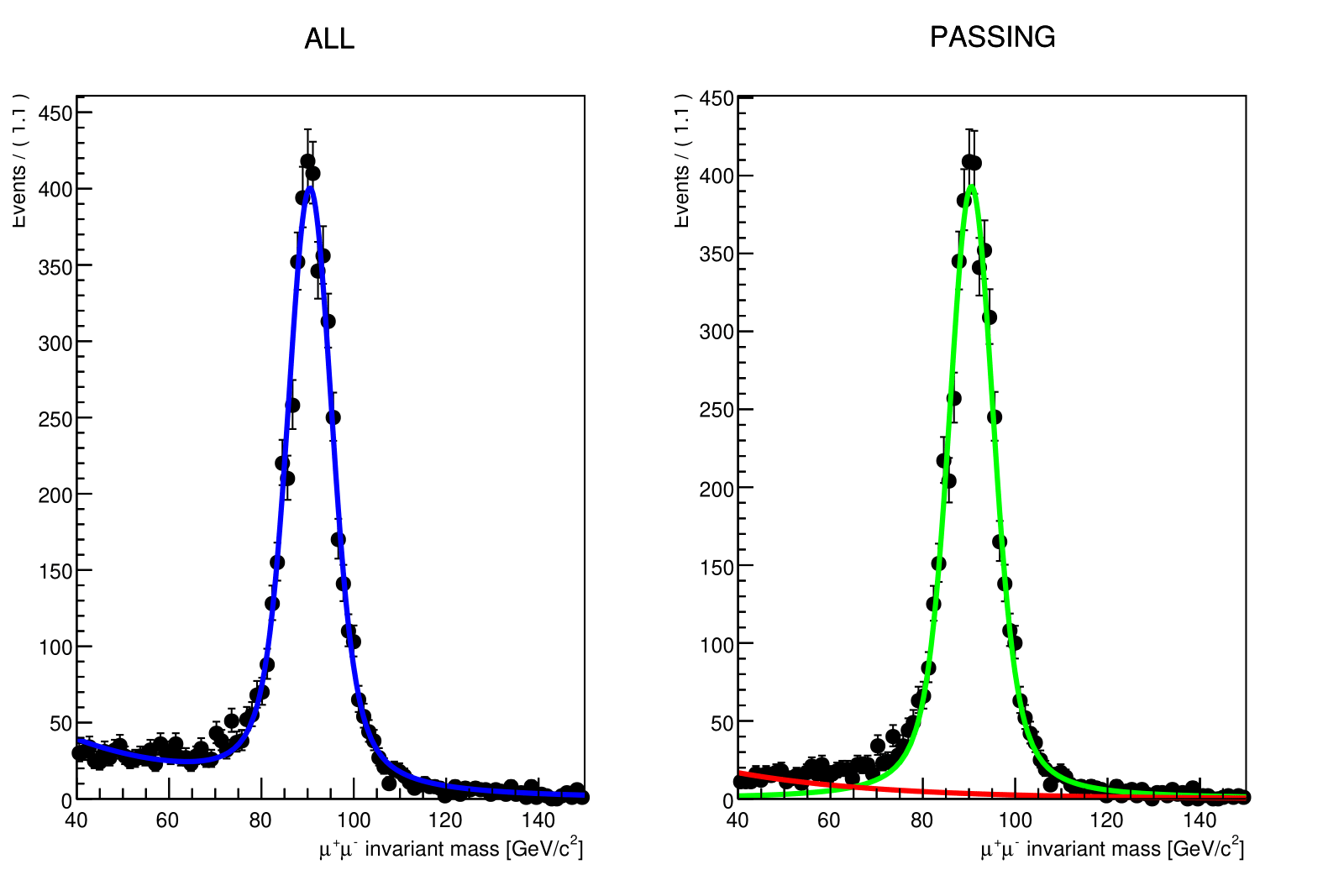
The fitting method

It consists on fitting the invariant mass of the tag & probe pairs, in the two categories: passing probes, and all probes. I.e., for the unbiased leg of the decay, one can apply a selection criteria (a set of cuts) and determine whether the object passes those criteria or not.

The procedure is applied after splitting the data in bins of a kinematic variable of the probe object (e.g. the traverse momentum, p_T); as such, the efficiency will be measured as a function of that quantity for each of the bins. So, in the picture below, on the left, let’s imagine that the p_T bin we are selecting is the one marked in red. But, of course, in that bin (like in the rest) you will have true Z decays as well as muon pairs from other processes (maybe QCD, for instance). The true decays would make up our signal, whereas the other events will be considered the background.

The fit, which is made in a different space (the invariant mass space) allows to statistically discriminate between signal and background. To compute the efficiency we simply divide the signal yield from the fits to the passing category by the signal yield from the fit of the inclusive (All) category. This approach is depicted in the middle and right-hand plots of the image below for the Y resonance.

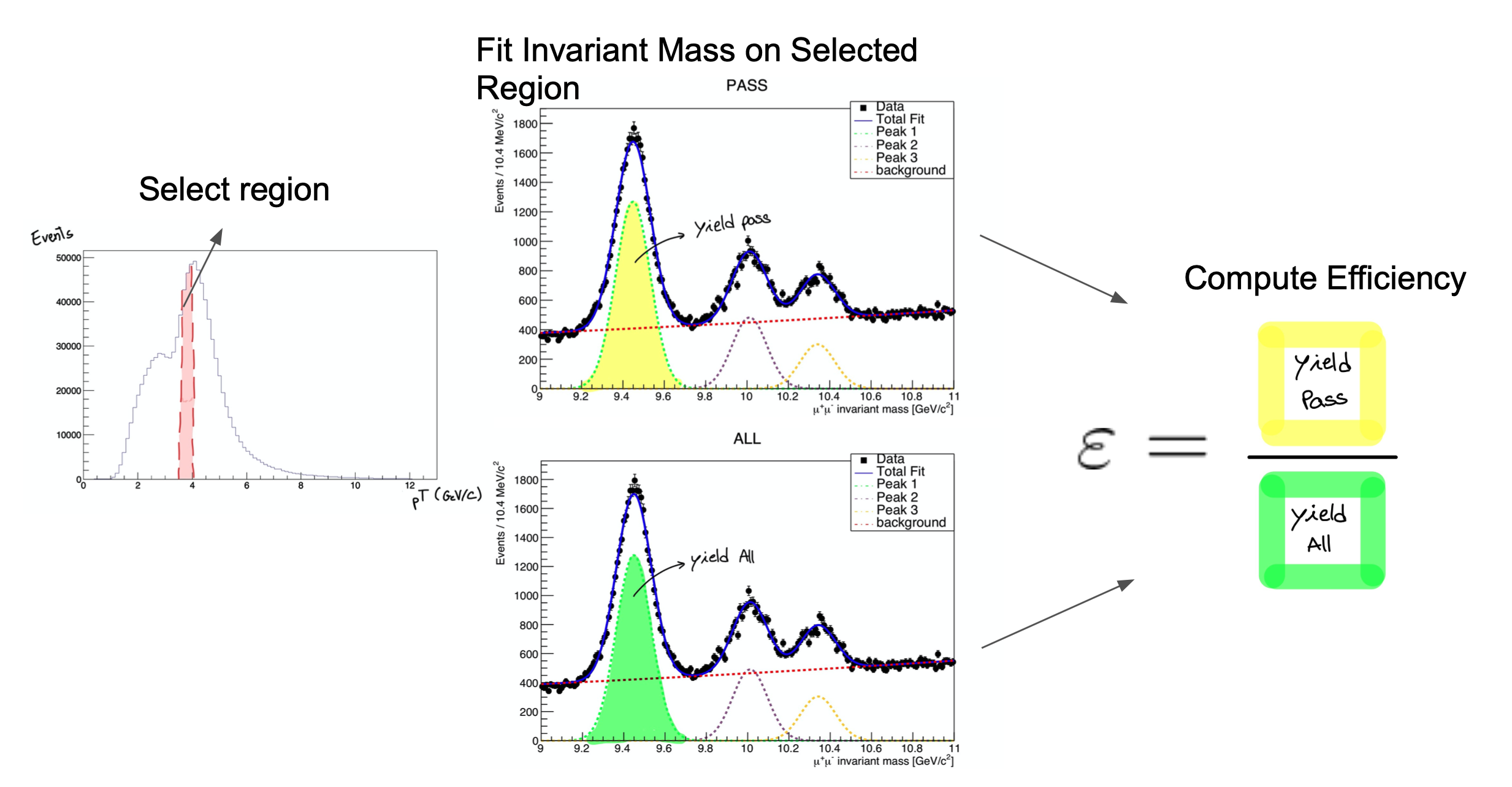
At the end of this section, then, you will have to make these fits for each bin in the range of interest. The dataset used in this exercise has been collected by the CMS experiment, in proton-proton collisions at the LHC. It contains 986100 entries (muon pair candidates) with an associated invariant mass. For each candidate, the transverse momentum (pt), rapidity(η) and azimuthal angle (φ) are stored, along with a binary flag probe_isTrkMatch, which is 1 in case the corresponding probe satisfied the track matching selection criteria and 0 in case it doesn’t.

Copy CMSDAS_TP inside CMSSW_10_6_18/src:

cp -r /eos/user/c/cmsdas/2023/short-ex-trk/CMSDAS_TP .

Exploring the content of the TP_Z_DATA.root and TP_Z_MC.root files, the StandAloneEvents tree has these variables in which we are interested in:

Variables to be checked

pair_mass

probe_isTrkMatch

probe_pt

probe_eta

probe_phi

We’ll start by calculating the efficiency as a function of the probe η. It is useful to have an idea of the distribution of the quantity we want to study. In order to do this, plot the invariant mass and the probe variables.

Now that you’re acquainted with the data, open the Efficiency.C file. We’ll start by choosing the desired bins for the rapidity. If you’re feeling brave, modify bins for our fit remembering that we need a fair amount of data in each bin (more events mean a better fit!). If not, we’ve left a suggestion in the Efficiency.C file. Start with the eta variable.

Now that the bins are set, we have defined the initial parameters for our fit. In this code, we execute a simultaneous fit using a Voigtian curve for the Z peak. For the background we use a Falling Exponential. The function used, doFit(), is implemented in the source file src/DoFit.cpp and it was based on the RooFit library. You can find generic tutorials for this library here. If you’re starting with RooFit you may also find this one particularly useful. You won’t need to do anything in src/DoFit.cpp but you can check it out if you’re curious.

To get the efficiency plot, we used the TEfficiency class from ROOT. You’ll see that in order to create a TEfficiency object, one of the constructors requires two TH1 objects, i.e., two histograms. One with all the probes and one with the passing probes.

The creation of these TH1 objects is taken care of by the src/make_hist.cpp code. Note that we load all these functions in the src area directly in header of the Efficiency.C code. Now that you understand what the Efficiency.C macro does, run your code with in a batch mode (-b) and with a quit-when-done switch (-q) root -q -b Efficiency.C.

When the execution finishes, you should have 2 new files. One on your working directory Histograms_Data.root and another one Efficiency_Run2018.root located at Efficiency_Result/eta. The second contains the efficiency we calculated, while the first file is used to re-do any unusuable fits. If you want, check out the PDF files under the Fit_Result/ directory, which contain the fitting results as the following one:

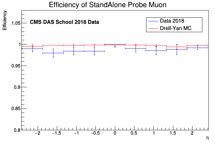
Now we must re-run the code, but before that, change IsMc value to TRUE. This will generate an efficiency for the simulated data, so that we can compare it with part of the 2018 run. If so, now uncomment Efficiency.C the following line:

// compare_efficiency(quantity, "Efficiency_Result/eta/Efficiency_Run2018.root", "Efficiency_Result/eta/Efficiency_MC.root");

and run the macro again. You should get something like the following result if you inspect the image at Comparison_Run2018_vs_MC_Efficiency.png:

If everything went well and you still have time to go, repeat this process for the two other variables, p_T and φ! In case you want to change one of the fit results, use the change_bin.cpp function commented in Efficiency.C. If you would like to explore the results having more statistics, use the samples in DATA/Z/ directory!

If you would like to play with the actual CMS tracking workflow have a look at the ntuple generator and the efficiency computation frameworks!

Looking at secondary vertices (continued)

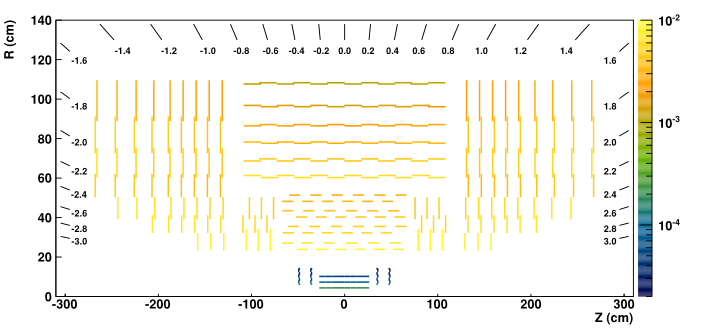
As an exercise, plot the positions of the vertices in a way that corresponds to the CMS half-view. That is, make a histogram like the following:

import math
import ROOT
rho_z_histogram = ROOT.TH2F("rho_z", "rho_z", 100, 0.0, 30.0, 100, 0.0, 10.0)

in which the horizontal axis will represent z, the direction parallel to the beamline, and the vertical axis will represent rho, the distance from the beamline, and fill it with (z, rho) pairs like this rho_z_histogram.Fill(z, rho).

Compute rho and z from the vertex objects:

events.toBegin()
for event in events:
    event.getByLabel("SecondaryVerticesFromLooseTracks", "Kshort", secondaryVertices)
    for vertex in secondaryVertices.product():
        rho_z_histogram.Fill(abs(vertex.vz()), math.sqrt(vertex.vx()**2 + vertex.vy()**2))

rho_z_histogram.Draw()

Question

What does the distribution tell you about CMS vertex reconstruction?

Half-view of CMS tracker (color indicates average number of hits):

Correlation between pile-up and number of clusters

import ROOT
import DataFormats.FWLite as fwlite
events = fwlite.Events("/eos/user/c/cmsdas/2023/short-ex-trk/run321167_ZeroBias_AOD.root")

clusterSummary = fwlite.Handle("ClusterSummary")

h = ROOT.TH2F("h", "h", 100, 0, 20000, 100, 0, 100000)

events.toBegin()
for event in events:
    event.getByLabel("clusterSummaryProducer", clusterSummary)
    cs = clusterSummary.product()
    try:
        h.Fill(cs.getNClus(cs.PIXEL),
               cs.getNClus(cs.PIXEL) + cs.getNClus(cs.STRIP))
    except TypeError:
        pass

c = ROOT.TCanvas("c", "c", 800, 800)
h.Draw()
h.Fit("pol1")
c.SaveAs("pileup_nclusters.png")

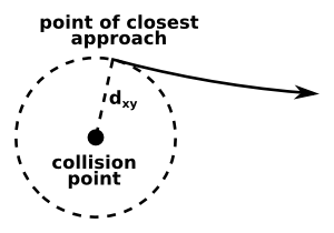
Harder questions: dxy biases

The dxy parameter is not simply a distance, it is a signed distance. A helical trajectory traces a circle in the plane transverse to the beamline, and the sign of dxy depends on whether the reference point is included inside of that circle our outside of it. You can change the reference point with which dxy is computed by passing a point or a beamspot as an argument:

print track.dxy()

-0.00082122773835

print track.dxy(ROOT.math.XYZPoint(0, 0, 0))

-0.00082122773835

print track.dxy(beamspot.product())

-0.00636893586021

Passing no parameter is equivalent to passing (0, 0, 0). Consider the following script:

import DataFormats.FWLite as fwlite
import ROOT

events = fwlite.Events("/eos/user/c/cmsdas/2023/short-ex-trk/run321167_ZeroBias_AOD.root")
tracks = fwlite.Handle("std::vector<reco::Track>")
beamspot = fwlite.Handle("reco::BeamSpot")

dxy_vs_phi_000 = ROOT.TProfile("dxy_vs_phi_000", "dxy_vs_phi_000", 100, -3.14, 3.14) 
dxy_vs_phi_beamspot = ROOT.TProfile("dxy_vs_phi_beamspot", "dxy_vs_phi_beamspot", 100, -3.14, 3.14) 

events.toBegin()
for event in events:
    event.getByLabel("generalTracks", tracks)
    event.getByLabel("offlineBeamSpot", beamspot)
    for track in tracks.product():
        dxy_vs_phi_000.Fill(track.phi(), track.dxy(ROOT.math.XYZPoint(0, 0, 0)))
        dxy_vs_phi_beamspot.Fill(track.phi(), track.dxy(beamspot.product()))

dxy_vs_phi_000.SetAxisRange(-0.2, 0.2, "Y")
dxy_vs_phi_beamspot.SetAxisRange(-0.2, 0.2, "Y")

c = ROOT.TCanvas("c", "c", 800, 800)
dxy_vs_phi_000.Draw()
dxy_vs_phi_beamspot.SetMarkerColor(ROOT.kRed)
dxy_vs_phi_beamspot.SetLineColor(ROOT.kRed)
dxy_vs_phi_beamspot.Draw("same")
c.SaveAs("beamspot.png")

It produces two plots, one of which shows a clear bias from the correct distribution (on average, dxy should be zero). This bias is not an problem with the detector, only a problem with interpreting it. Can you explain the origin of the bias, including its shape with respect to phi?

Below, there is a figure that might help. It is also useful to draw sketches for yourself.

Bonus Exercise: µµTrkTrk reconstruction in MiniAOD

Please have a look to the instruction at the repository at https://github.com/CMSTrackingPOG/2mu2trk_exercise/blob/main/README.md.

Please notice that it requires a newer CMSSW version!

Documentation

Key Points

At this point it is extremely important to look at the documentation to find out moreabout the Tracking Physics Object Group (TRK POG) tasks.

CMS DAS 2023 Tracking and Vertexing Short Exercise

CMS Data Analysis School Tracking and Vertexing Short Exercise - The five basic track variables

Overview

The five basic track parameters

Accessing track variables

C++ version

Track quality variables

C++ version

Question 1

Answer

Track information in MiniAOD

Track information in PFCandidates collection

Question 2

Answer

Key Points

CMS Data Analysis School Tracking and Vertexing Short Exercise - Tracks as particles

Overview

Question 1

Answer

Additional information

Question 2

More…

Key Points

CMS Data Analysis School Tracking and Vertexing Short Exercise - Constructing vertices from tracks

Overview

Running the vertex reconstruction

Looking at secondary vertices

Question 1

Answer (don’t look until you’ve tried it!)

Question 2

More

Question 3

Question 4

Answer

Question 5

Secondary vertices in MiniAOD

Question 6

Answer

Basic distributions of primary vertices

Steps of primary vertex reconstruction

Question 7

Answer

Solution

Question 8

Answer

More exercises…

Answer

Primary vertices improve physics results

Question 9

Answer

Solution

Solution

Key Points

CMS Data Analysis School Tracking and Vertexing Short Exercise - Appendix

Overview

LXR: a tool to search through CMSSW code

Further useful code references

Tracking efficiency performance via the Tag and Probe technique

What is “tag” and “probe”?

How do we calculate the efficiency?

The fitting method

Variables to be checked

Looking at secondary vertices (continued)

Question

Correlation between pile-up and number of clusters

Harder questions: dxy biases

Bonus Exercise: µµTrkTrk reconstruction in MiniAOD

Documentation

Key Points